Normalization in Seaborn Bar Plots (Reduce Outliers)

Normalization is transforming your data onto a common scale without distorting differences in the ranges of values.

In this tutorial, you’ll learn various normalization methods such as Min-Max Normalization, Z-Score Normalization, Decimal Scaling, Log Transformation, and Quantile Normalization.

You’ll understand how to implement these methods in Python and apply them to Seaborn bar plots.

Also, we’ll see the differences between normalized and unnormalized plots through side-by-side comparisons.

 

 

Unnormalized Bar Plots in Seaborn

First, let’s import the necessary libraries and create a sample dataset.

import seaborn as sns
import matplotlib.pyplot as plt
import pandas as pd
data = {
    'Region': ['North', 'South', 'East', 'West', 'North', 'South', 'East', 'West'],
    'Data Usage': [500, 600, 550, 450, 300, 400, 350, 500]
}
df = pd.DataFrame(data)

Now, let’s create a basic bar plot using Seaborn.

sns.barplot(x='Region', y='Data Usage', data=df)
plt.show()

Output:

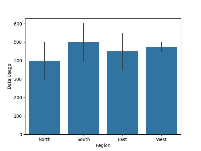
Why It’s Misleading: The issue here is that the plot shows average data usage per region, but it doesn’t account for the varying number of customers in each region.

This can lead to incorrect interpretations, especially when comparing regions.

In the next section, you’ll see how normalization can address this issue.

 

Min-Max Normalization (Scaling)

Now, let’s implement Min-Max Normalization on our dataset. Min-Max Normalization brings all values into the range [0,1].

We’ll apply Min-Max Scaling to the ‘Data Usage’ column in our dataset.

from sklearn.preprocessing import MinMaxScaler
scaler = MinMaxScaler()
data_usage_reshaped = df['Data Usage'].values.reshape(-1, 1)
df['Normalized Data Usage'] = scaler.fit_transform(data_usage_reshaped)
print(df.head())

Output:

  Region  Data Usage  Normalized Data Usage
0  North         500               0.666667
1  South         600               1.000000
2   East         550               0.833333
3   West         450               0.500000
4  North         300               0.000000

Each value in this column is a scaled version of the original ‘Data Usage’, now within the range [0,1].

Let’s plot the normalized data:

sns.barplot(x='Region', y='Normalized Data Usage', data=df)
plt.show()

Output:

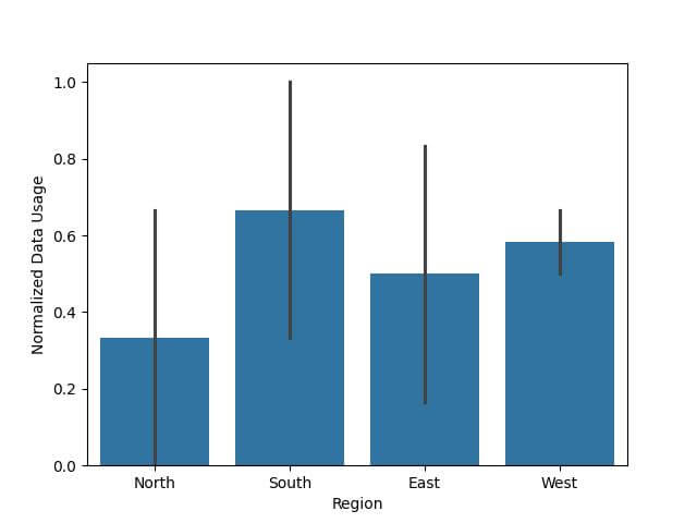
This method of normalization ensures that you’re comparing data on an equal footing.

 

Z-Score Normalization (Standardization)

Z-Score Normalization, also known as Standardization involves re-scaling data to have a mean of 0 and a standard deviation of 1.

This method is useful when dealing with data that follows a Gaussian distribution.

Let’s apply Z-Score Normalization to the ‘Data Usage’ in our dataset.

from scipy.stats import zscore
df['Z-Score Normalized Data Usage'] = zscore(df['Data Usage'])
print(df.head())

Output:

  Region  Data Usage  Z-Score Normalized Data Usage
0  North         500                       0.460566
1  South         600                       1.513289
2   East         550                       0.986928
3   West         450                      -0.065795
4  North         300                      -1.644879

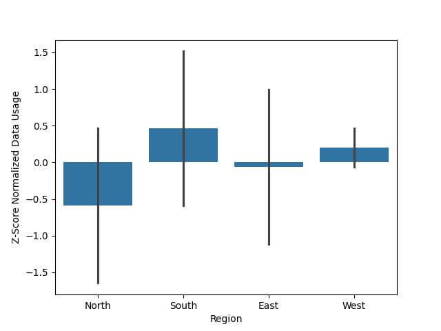
Here, each value represents how many standard deviations away from the mean the original ‘Data Usage’ value was.

Next, let’s visualize this standardized data:

sns.barplot(x='Region', y='Z-Score Normalized Data Usage', data=df)
plt.show()

Output:

 

Decimal Scaling

Decimal Scaling is a normalization method where you divide each data point by 10 raised to the maximum number of digits in the dataset.

This method is straightforward and effective for reducing the scale of values without distorting differences in the ranges of values.

Let’s apply Decimal Scaling to our ‘Data Usage’ data.

max_digits = len(str(max(df['Data Usage'])))
df['Decimal Scaled Data Usage'] = df['Data Usage'] / (10 ** max_digits)
print(df.head())

Output:

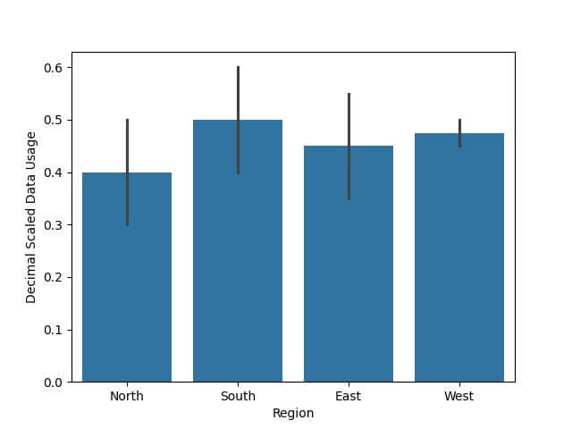
  Region  Data Usage  Decimal Scaled Data Usage
0  North         500                       0.50
1  South         600                       0.60
2   East         550                       0.55
3   West         450                       0.45
4  North         300                       0.30

Now, let’s visualize this:

sns.barplot(x='Region', y='Decimal Scaled Data Usage', data=df)
plt.show()

Output:

 

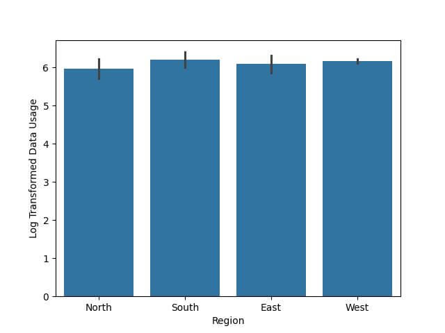
Log Transformation

Log Transformation is a method used to manage skewed data and reduce the effect of outliers.

By applying a logarithmic scale to your data, you can transform a highly skewed distribution into a more normal distribution, making it easier to analyze and visualize.

Let’s apply a Log Transformation to the ‘Data Usage’ in our dataset.

import numpy as np
df['Log Transformed Data Usage'] = np.log(df['Data Usage'] + 1)  # Adding 1 to avoid log(0)
print(df.head())

Output:

  Region  Data Usage  Log Transformed Data Usage
0  North         500                    6.216606
1  South         600                    6.398595
2   East         550                    6.311735
3   West         450                    6.111467
4  North         300                    5.707110

Now, let’s visualize this transformed data:

sns.barplot(x='Region', y='Log Transformed Data Usage', data=df)
plt.show()

Output:

 

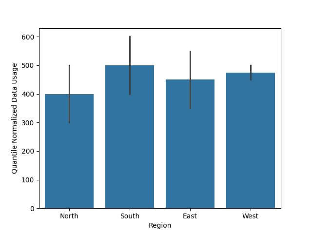
Quantile Normalization

Quantile Normalization is a method used to make two distributions identical in statistical properties.

This method is useful when the distributions of the data are known to be different and you need to bring them to a common scale.

Let’s apply Quantile Normalization to the ‘Data Usage’ column in our dataset.

First, we need to sort the data, average the sorted values across samples for the same quantile, and then assign these averaged values back to the original data based on their rank.

def quantile_normalize(series):
    sorted_values = series.sort_values()
    ranks = series.rank(method='first').astype(int) - 1
    normalized = sorted_values.values[ranks]
    return pd.Series(normalized, index=series.index)
df['Quantile Normalized Data Usage'] = quantile_normalize(df['Data Usage'])
print(df.head())

Output:

  Region  Data Usage  Quantile Normalized Data Usage
0  North         500                             500
1  South         600                             600
2   East         550                             550
3   West         450                             450
4  North         300                             300

Now, let’s visualize the quantile normalized data:

sns.barplot(x='Region', y='Quantile Normalized Data Usage', data=df)
plt.show()

Output:

 

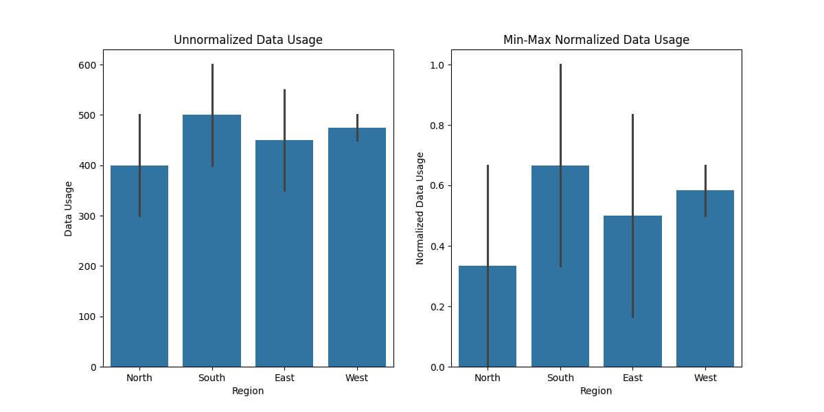
Comparing Normalized and Unnormalized Plots

Let’s create side-by-side plots for our dataset, comparing the original unnormalized ‘Data Usage’ with one of the normalized versions, say, Min-Max Normalization.

plt.figure(figsize=(12, 6))

# Plot 1: Unnormalized Data
plt.subplot(1, 2, 1)  # 1 row, 2 columns, 1st subplot
sns.barplot(x='Region', y='Data Usage', data=df)
plt.title('Unnormalized Data Usage')

# Plot 2: Min-Max Normalized Data
plt.subplot(1, 2, 2)  # 1 row, 2 columns, 2nd subplot
from sklearn.preprocessing import MinMaxScaler
scaler = MinMaxScaler()
data_usage_reshaped = df['Data Usage'].values.reshape(-1, 1)
df['Normalized Data Usage'] = scaler.fit_transform(data_usage_reshaped)
sns.barplot(x='Region', y='Normalized Data Usage', data=df)
plt.title('Min-Max Normalized Data Usage')
plt.show()

Output:

 

Choosing an Appropriate Normalization Range

Before choosing a normalization range, you must understand your data’s distribution:

• Skewed Data: If data is skewed, consider normalization methods like Log Transformation or Z-Score Normalization, which are less sensitive to outliers.
• Linear Distribution: For linearly distributed data, Min-Max Normalization is often effective.
• Presence of Outliers: In data with outliers, Z-Score Normalization or Log Transformation is more appropriate than Min-Max Normalization.

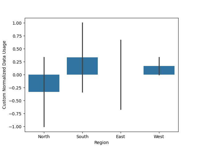
Implementing a Custom Normalization Range

You can implement a custom normalization range based on your specific requirements.

def custom_normalize(data, new_min, new_max):
    old_min, old_max = data.min(), data.max()
    return (data - old_min) / (old_max - old_min) * (new_max - new_min) + new_min

# Example: Normalizing to a range of [-1, 1]
df['Custom Normalized Data Usage'] = custom_normalize(df['Data Usage'], -1, 1)

Now, let’s visualize the normalized data:

sns.barplot(x='Region', y='Custom Normalized Data Usage', data=df)
plt.show()

Output: