Remove Outliers from Histogram Visualizations in Python
In this tutorial, you’ll learn various methods to identify and remove outliers from your Seaborn histogram data.
We’ll explore methods like the Z-score method, Interquartile Range (IQR) method, and Standard Deviation method.
Impact of Outliers on Data Visualization
We’ll start by generating a sample dataset with outliers.
import numpy as np
import matplotlib.pyplot as plt
np.random.seed(0)
data = np.random.normal(50, 15, 1000)

# Introducing outliers
data_with_outliers = np.append(data, [200, 205, 210])
plt.hist(data_with_outliers, bins=30, color='skyblue', edgecolor='black')
plt.title('Histogram with Outliers')
plt.xlabel('Value')
plt.ylabel('Frequency')
plt.show()
Code Output:
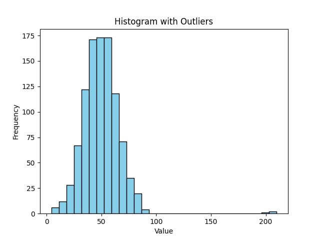
In this histogram, you can see how the outliers (values around 200) create a skewed view of the data distribution.
The majority of the data is centered around 50, but the presence of extreme values distorts the scale, making it harder to analyze the bulk of the data effectively.
Using Z-score Method
The Z-score method measures how many standard deviations away a data point is from the mean. Typically, data points with a Z-score greater than 3 or less than -3 are considered outliers.
We’ll calculate the Z-scores for each data point and then filter out the outliers.
from scipy import stats

# Calculating Z-scores
z_scores = stats.zscore(data_with_outliers)

# Filtering data without outliers
data_without_outliers = data_with_outliers[(z_scores > -3) & (z_scores < 3)]
plt.hist(data_without_outliers, bins=30, color='lightgreen', edgecolor='black')
plt.title('Histogram without Outliers')
plt.xlabel('Value')
plt.ylabel('Frequency')
plt.show()
Code Output:
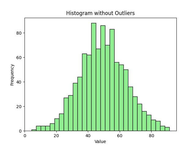
The data is now more centrally clustered, offering a clearer view of the true distribution.
Using IQR (Interquartile Range) Method
Another method for identifying and removing outliers is the Interquartile Range (IQR) method.
The IQR is the difference between the 75th percentile (Q3) and the 25th percentile (Q1) of the data.
Outliers are typically defined as observations that fall below Q1 – 1.5_IQR or above Q3 + 1.5_IQR.
# Calculating Q1, Q3, and IQR
Q1 = np.percentile(data_with_outliers, 25)
Q3 = np.percentile(data_with_outliers, 75)
IQR = Q3 - Q1

# Filtering data based on IQR
data_iqr_filtered = data_with_outliers[(data_with_outliers >= (Q1 - 1.5 * IQR)) & (data_with_outliers <= (Q3 + 1.5 * IQR))]
plt.hist(data_iqr_filtered, bins=30, color='lightcoral', edgecolor='black')
plt.title('Histogram after IQR Filtering')
plt.xlabel('Value')
plt.ylabel('Frequency')
plt.show()
Code Output:
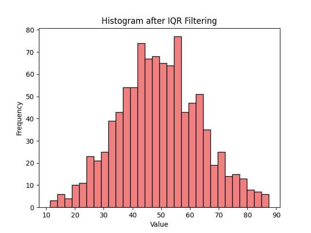
This approach using the IQR method has eliminated extreme values.
Using Standard Deviation Method
In this method, we consider data points that lie beyond a certain number of standard deviations from the mean as outliers.
A common practice is to exclude data points that are more than two or three standard deviations away from the mean.
# Calculating mean and standard deviation
mean = np.mean(data_with_outliers)
std_deviation = np.std(data_with_outliers)

# Defining the threshold for outliers
threshold = 3 * std_deviation

# Filtering out outliers
data_std_filtered = data_with_outliers[(data_with_outliers > (mean - threshold)) & (data_with_outliers < (mean + threshold))]
plt.hist(data_std_filtered, bins=30, color='goldenrod', edgecolor='black')
plt.title('Histogram after Standard Deviation Filtering')
plt.xlabel('Value')
plt.ylabel('Frequency')
plt.show()
Code Output:
Ensuring Data Integrity Post Outlier Removal
After removing outliers from your dataset, it’s important to ensure that the integrity of your data remains intact.
This means verifying that the data still accurately reflects the case you’re analyzing.
Here are steps to validate data integrity post outlier removal:
- Statistical Summary: Examine basic statistical measures before and after outlier removal.
- Distribution Analysis: Compare the distributions pre and post outlier removal.
- Consistency Check: Ensure that the data still aligns with expected patterns or known benchmarks.
Let’s apply these steps to our dataset:
# Statistical Summary before outlier removal
original_stats = {
    "Mean": np.mean(data_with_outliers),
    "Standard Deviation": np.std(data_with_outliers),
    "Min": np.min(data_with_outliers),
    "Max": np.max(data_with_outliers)
}

# Statistical Summary after outlier removal using Standard Deviation method
filtered_stats = {
    "Mean": np.mean(data_std_filtered),
    "Standard Deviation": np.std(data_std_filtered),
    "Min": np.min(data_std_filtered),
    "Max": np.max(data_std_filtered)
}

print("Original Data Statistics:", original_stats)
print("Filtered Data Statistics:", filtered_stats)
Code Output:
Original Data Statistics: {'Mean': 49.78678902058531, 'Standard Deviation': 17.054922584770093, 'Min': 4.307854178001101, 'Max': 210.0}
Filtered Data Statistics: {'Mean': 49.32114938764706, 'Standard Deviation': 14.805497380035387, 'Min': 4.307854178001101, 'Max': 91.39032671032373}
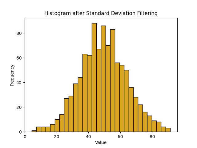
The output shows that the mean and standard deviation have become more representative of the central data points after outlier removal.
Mokhtar is the founder of LikeGeeks.com. He is a seasoned technologist and accomplished author, with expertise in Linux system administration and Python development. Since 2010, Mokhtar has built an impressive career, transitioning from system administration to Python development in 2015. His work spans large corporations to freelance clients around the globe. Alongside his technical work, Mokhtar has authored some insightful books in his field. Known for his innovative solutions, meticulous attention to detail, and high-quality work, Mokhtar continually seeks new challenges within the dynamic field of technology.