Plot Seaborn Line Plot with Mean and Standard Deviation

To plot a Seaborn line plot with mean and standard deviation:

• Use sns.lineplot() from Seaborn, specify your x and y axes data.
• Set estimator=np.mean to plot the mean of your y-values, and errorbar='sd' to display the standard deviation as a shaded area around the line.

In this tutorial, we’ll learn how to compute the mean and standard deviation and visualize these statistics in a line plot using Seaborn.

 

 

Mean Calculation

Grouped Data

For grouped data, where you need to calculate the mean of a specific column based on the grouping of another column, use the groupby method combined with mean.

import pandas as pd
data = {
    'Week': [1, 1, 2, 2, 3, 3],
    'Data_Usage': [500, 450, 520, 480, 550, 530]
}
df = pd.DataFrame(data)
mean_usage = df.groupby('Week')['Data_Usage'].mean()
print(mean_usage)

Output:

Week
1    475.0
2    500.0
3    540.0
Name: Data_Usage, dtype: float64

This output shows the average data usage for each week.

Ungrouped Data

For ungrouped data, where the dataset is a simple list or a series without the need for grouping, you can calculate the mean using the mean method.

total_data_usage = df['Data_Usage']
mean_total_usage = total_data_usage.mean()
print(mean_total_usage)

Output:

505.0

Here, the output represents the average data usage over the entire dataset.

 

Standard Deviation Calculation

Grouped Data

For grouped data, you can calculate the standard deviation for each group in a similar way as you did for the mean.

# Calculating standard deviation of data usage per week
std_deviation_usage = df.groupby('Week')['Data_Usage'].std()
print(std_deviation_usage)

Output:

Week
1    35.355339
2    28.284271
3    14.142136
Name: Data_Usage, dtype: float64

Lower values indicate more consistency in usage within that week.

Ungrouped Data

For ungrouped data, where you’re looking at the overall variability of a single dataset without categorization, use the std method.

std_dev_total_usage = total_data_usage.std()
print(std_dev_total_usage)

Output:

36.193922141707716

This number signifies the spread of data usage across the entire dataset.

 

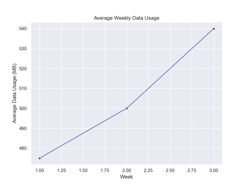
Plot Mean Values

Let’s plot the mean data usage we calculated earlier.

import seaborn as sns
import matplotlib.pyplot as plt

# Resetting the index to use 'Week' as a column
mean_usage_df = mean_usage.reset_index()
sns.set_theme(style="darkgrid")
plt.figure(figsize=(8, 6))
sns.lineplot(x='Week', y='Data_Usage', data=mean_usage_df, marker='o')
plt.title('Average Weekly Data Usage')
plt.xlabel('Week')
plt.ylabel('Average Data Usage (MB)')
plt.show()

Output:

 

Add Error Bars to Represent Standard Deviation

To add error bars for standard deviation, we can use the estimator and errorbar parameters instead of passing the standard deviation values directly.

import matplotlib.pyplot as plt
import seaborn as sns
import numpy as np
plt.figure(figsize=(8, 6))
sns.lineplot(x='Week', y='Data_Usage', data=df, marker='o', 
             estimator=np.mean, errorbar='sd')
plt.title('Weekly Data Usage with Standard Deviation')
plt.xlabel('Week')
plt.ylabel('Data Usage (MB)')
plt.show()

Output:

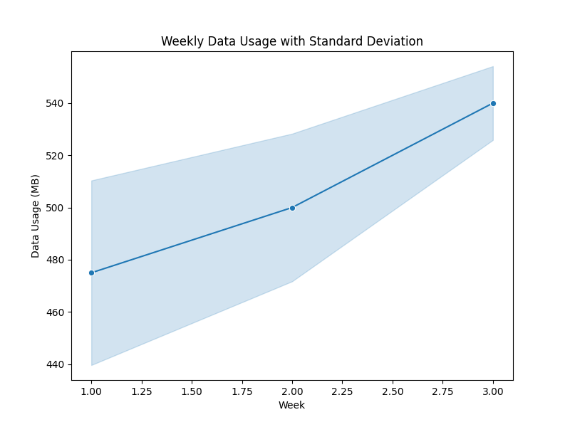
The plot shows the mean weekly data usage with a shaded area around each line representing the standard deviation.