Create Seaborn Line Plot from Pandas Multiindex DataFrame
In this tutorial, you will learn how to create Seaborn line plot from a Pandas MultiIndex DataFrame.
We’ll cover various methods to visualize this data, including groupby() for aggregated views, looping over MultiIndex levels for detailed analyses, and using Seaborn FacetGrid for creating multi-plot grids.
Convert MultiIndex to Regular Columns
Before plotting a multiindex DataFrame, we need to flatten the multiindex to regular columns to be able to plot them.
Using reset_index()
The Pandas reset_index() converts the MultiIndex into regular columns which makes the DataFrame suitable for plotting with Seaborn.
import pandas as pd
import numpy as np
import seaborn as sns
import matplotlib.pyplot as plt
np.random.seed(0)
dates = pd.date_range('2024-01-01', periods=90)
regions = ['North', 'South', 'East', 'West']
idx = pd.MultiIndex.from_product([dates, regions], names=['Date', 'Region'])
df = pd.DataFrame({
    'Calls': np.random.randint(100, 500, size=len(idx)),
    'DataUsage': np.random.rand(len(idx)) * 100,
    'Revenue': np.random.randint(200, 1000, size=len(idx))
}, index=idx)
df_reset = df.reset_index()
Output:
            Date Region  Calls   DataUsage  Revenue
0     2023-01-01  North    ...    ...       ...
...   ...         ...      ...    ...       ...
359   2023-03-31  West     ...    ...       ...
Next, we create a line plot using Seaborn to visualize the ‘Revenue’ trends over time for each region.
plt.figure(figsize=(12, 6))
sns.lineplot(data=df_reset, x='Date', y='Revenue', hue='Region')
plt.title('Revenue Trends Over Time by Region')
plt.xlabel('Date')
plt.ylabel('Revenue')
plt.xticks(rotation=45)
plt.tight_layout()
plt.show()
Output:
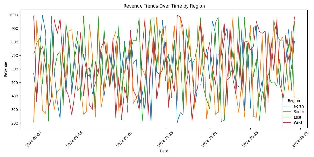
The hue parameter in sns.lineplot allows us to differentiate the regions with distinct colors.
Using unstack()
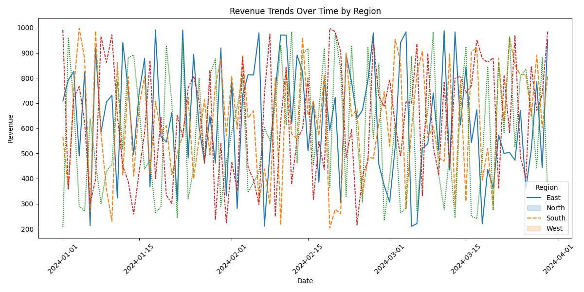
You can use unstack() to transform data from a multi-level or hierarchical index format into columns.
Let’s plot the ‘Revenue’ trends over time for each region.
df_pivoted = df['Revenue'].unstack(level='Region')
plt.figure(figsize=(12, 6))
sns.lineplot(data=df_pivoted)
plt.title('Revenue Trends Over Time by Region')
plt.xlabel('Date')
plt.ylabel('Revenue')
plt.xticks(rotation=45)
plt.legend(title='Region', labels=df_pivoted.columns)
plt.tight_layout()
plt.show()
Output:
GroupBy Plotting
You can use Pandas groupby() if you want to analyze aggregated values over specific dimensions.
Let’s say we’re interested in the average daily revenue for each region.
grouped_df = df.groupby(level=['Date', 'Region']).mean()
grouped_df_reset = grouped_df.reset_index()
plt.figure(figsize=(12, 6))
sns.lineplot(data=grouped_df_reset, x='Date', y='Revenue', hue='Region')
plt.title('Average Daily Revenue Trends by Region')
plt.xlabel('Date')
plt.ylabel('Average Revenue')
plt.xticks(rotation=45)
plt.tight_layout()
plt.show()
Output:
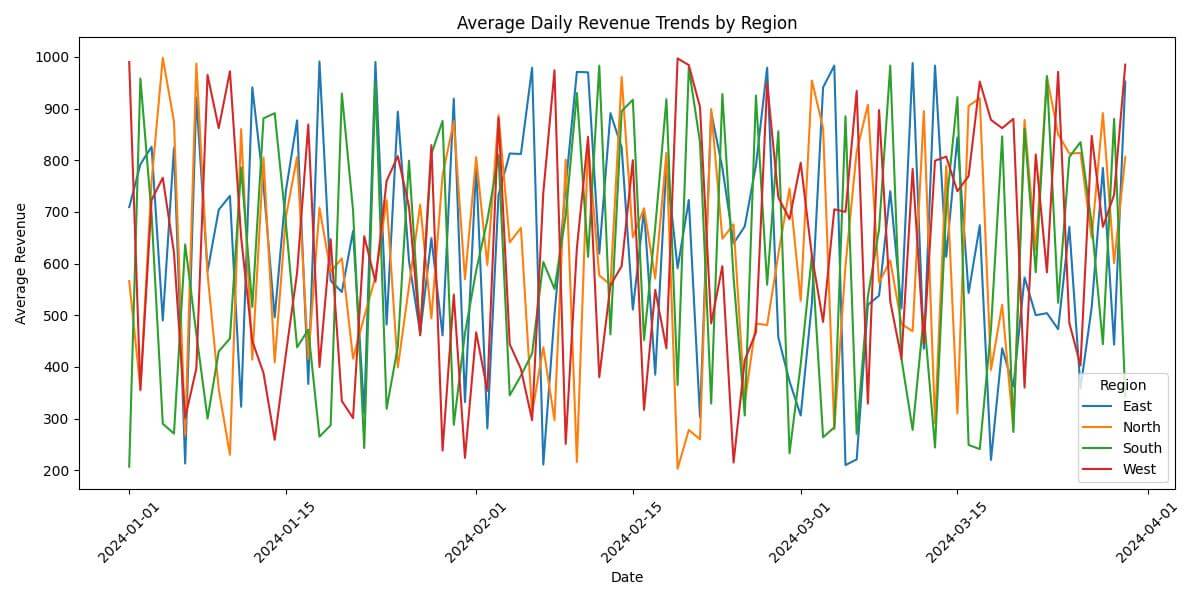
In this code, groupby(level=['Date', 'Region']).mean() calculates the average revenue for each day and region.
Looping Over MultiIndex Levels
Let’s say we want to create separate line plots for each region.
Here’s how you can loop over one level of the MultiIndex and create a line plot for each region:
for region in df.index.get_level_values('Region').unique():
    plt.figure(figsize=(12, 6))
    region_data = df.xs(region, level='Region')
    sns.lineplot(data=region_data, x=region_data.index, y='Revenue')
    plt.title(f'Revenue Trends for {region} Region')
    plt.xlabel('Date')
    plt.ylabel('Revenue')
    plt.xticks(rotation=45)
    plt.tight_layout()
    plt.show()
Output:
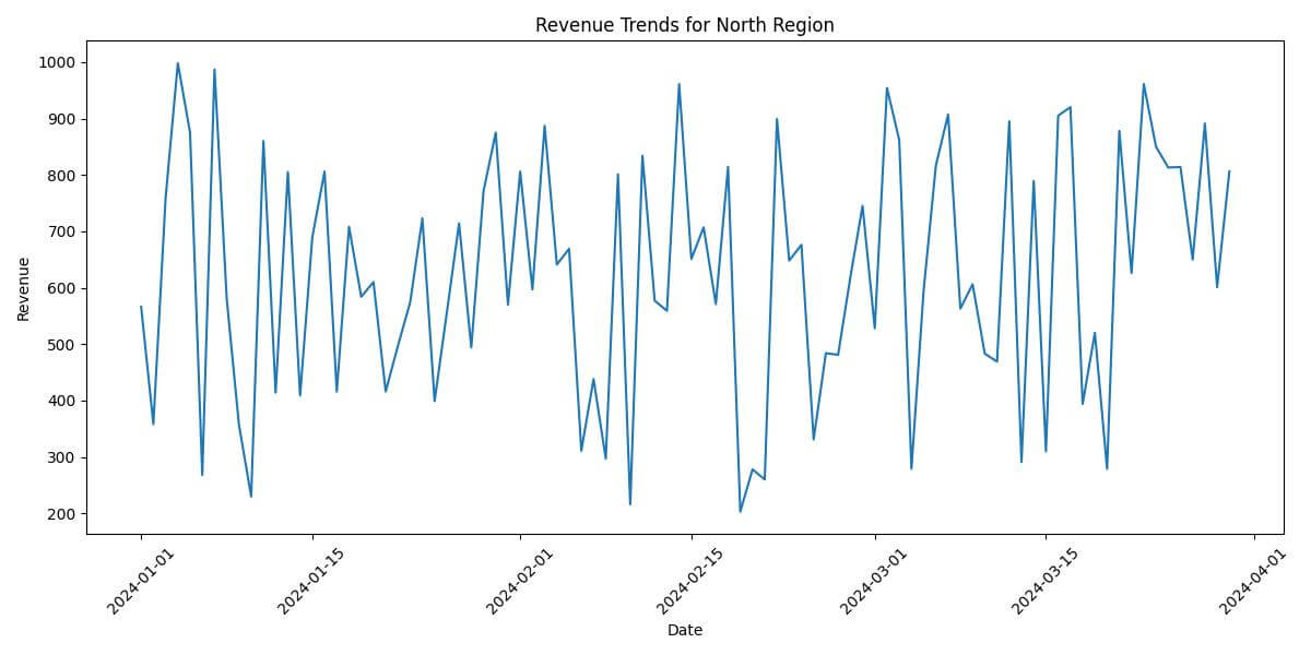
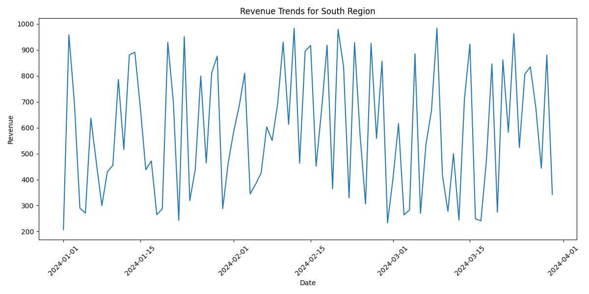
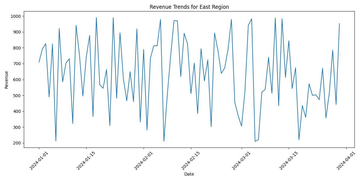
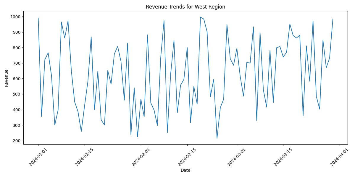
In this code, df.index.get_level_values('Region').unique() retrieves unique values from the ‘Region’ level of the MultiIndex.
The xs() method is then used to select data for each specific region.
Each iteration of the loop generates a line plot for that region’s revenue over time.
FacetGrid for Multi-Plot Grids
Seaborn FacetGrid allows you to create a grid of plots based on the levels of a MultiIndex.
Here’s how you can create a grid of line plots, each corresponding to a different region:
df_reset = df.reset_index()
g = sns.FacetGrid(df_reset, col="Region", hue="Region", col_wrap=2, height=4, aspect=1.5)
g.map(sns.lineplot, "Date", "Revenue")

g.fig.suptitle('Revenue Trends by Region', y=1.02)
g.set_axis_labels('Date', 'Revenue')
g.set_xticklabels(rotation=45)
g.add_legend()
plt.tight_layout()
plt.show()
Output:
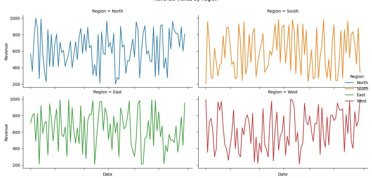
The map function applies the sns.lineplot to each subplot, plotting the ‘Revenue’ against ‘Date’.
The col_wrap parameter determines how many plots are in each row of the grid, and height and aspect control the size of each plot.
Mokhtar is the founder of LikeGeeks.com. He is a seasoned technologist and accomplished author, with expertise in Linux system administration and Python development. Since 2010, Mokhtar has built an impressive career, transitioning from system administration to Python development in 2015. His work spans large corporations to freelance clients around the globe. Alongside his technical work, Mokhtar has authored some insightful books in his field. Known for his innovative solutions, meticulous attention to detail, and high-quality work, Mokhtar continually seeks new challenges within the dynamic field of technology.