NumPy Meshgrid From Zero To Hero
Python’s NumPy is the most commonly used library for working with array/matrix data.
A matrix can be viewed as a 2-dimensional ‘grid’ of values, where the position of each value in the grid is given by a pair of values (i, j).
These values represent the row and column number of that value in the grid.
In this tutorial, we will understand how we can create such grids and work with them using the NumPy library in Python.
- 1 What is a meshgrid?
- 2 What are the benefits of meshgrid?
- 3 Creating a 2D NumPy meshgrid from two 1D arrays
- 4 Creating a NumPy meshgrid with sparse=True
- 5 Creating a NumPy meshgrid of polar coordinates
- 6 NumPy meshgrid with ‘matrix indexing’
- 7 Flip a NumPy meshgrid
- 8 Creating Meshgrid with NumPy matrices
- 9 Creating a 3-dimensional meshgrid
- 10 Creating a 3D surface plot using NumPy meshgrid
- 11 Avoiding NumPy meshgrid memory error
- 12 Conclusion
What is a meshgrid?
The term meshgrid is made up of two words – ‘mesh’ and ‘grid’, both of which in general
refer to ‘a network’ or ‘an interlaced structure’ or an ‘arrangement’ of equally spaced values
The Cartesian coordinate system is a classic example of this.
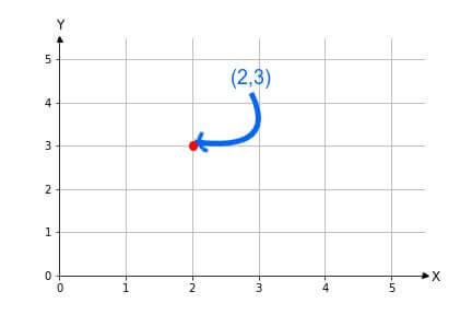
As shown in the image, each position is referred to by an ordered pair of indices or X and Y coordinates.
Using NumPy’s meshgridmethod, we will create such ordered pairs to construct a grid.
What are the benefits of meshgrid?
Meshgrids can be useful in any application where we need to construct a well-defined 2D or even multi-dimensional space, and where we need the ability to refer to each position in the space.
However, the most prominent application of meshgrids is seen in data visualization. To visualize patterns in data, or to plot a function in a 2D or a 3D space, meshgrids play an important role by creating ordered pairs of dependent variables.
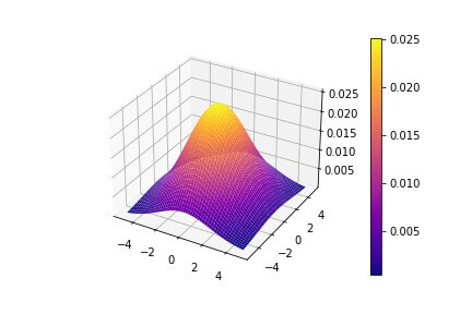
Here are the two examples of such data visualization achieved using meshgrid as an intermediary step.
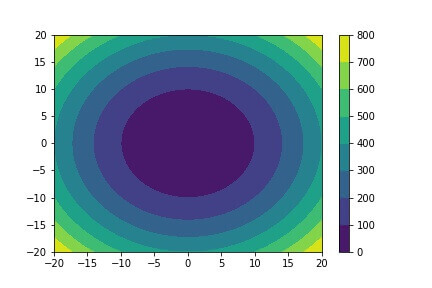
The first plot shows a contour plot of circles, with varying radii and centers at (0,0).
The second plot is a 3D Gaussian surface plot.
These plots use co-ordinates generated using numpy.meshgrid.
Creating a 2D NumPy meshgrid from two 1D arrays
Let us begin with a simple example of using meshgrid.
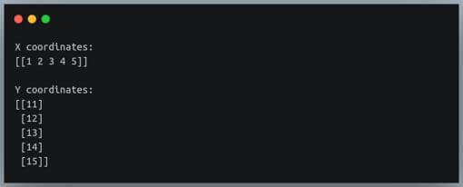
We want to create a 5×5 cartesian grid, with x coordinates ranging from 1 to 5, and y coordinates ranging from 11 to 15.
That means the ordered pairs of (x, y) coordinates will begin from (1,11) and go on till (5,15).
We also need to separately store the x and y coordinates of each position in the grid.
X = np.array([1,2,3,4,5])
Y = np.array([11, 12, 13, 14, 15])
xx, yy = np.meshgrid(X,Y)
print("X coordinates:\n{}\n".format(xx))
print("Y coordinates:\n{}".format(yy))
Output:
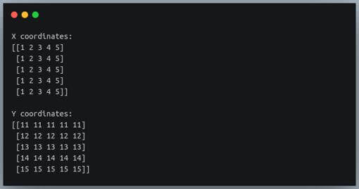
We get two NumPy arrays as output, each of shape 5×5.
The first array represents the x coordinates of each position in the grid, while the second array represents the corresponding y coordinates.
If you take ordered pairs of the values at the same positions in the two arrays, you will get (x, y) coordinates of all positions in our intended grid.
For example, the values at position [0,0] in the two arrays represent the position (1,11). Those at [0,1] represent the position (2,11), and so on.
Creating a NumPy meshgrid with sparse=True
If you look closely at the output of np.meshgrid in the previous example, the first output array xx has the same 1D array repeated row-wise, and the second output array yy has the same array repeated column-wise.
So to construct a grid, we only need information about the 1D arrays being repeated and their orientation.
This is achieved by specifying the value of parameter ‘sparse‘ as ‘True’
As the name suggests, it returns a ‘sparse’ representation of the grid.
Let us reconstruct the same grid with sparse=True
X = np.array([1,2,3,4,5])
Y = np.array([11, 12, 13, 14, 15])
xx, yy = np.meshgrid(X,Y, sparse=True)
print("X coordinates:\n{}\n".format(xx))
print("Y coordinates:\n{}".format(yy))
Output:
Now the output arrays are no longer of the shape 5×5. The xx array is of shape 1×5, and the yy array of shape 5×1
Note that this does not affect any further computation of values on the grid.
For instance, if you want to compute some function on the grid values, you can do so using the sparse representation and get a 5×5 output.
This is possible due to the broadcasting of NumPy arrays
Creating a NumPy meshgrid of polar coordinates
So far, we have seen how we can generate a grid of coordinates in the Cartesian coordinate system.
However, there also exists another coordinate system called the ‘Polar coordinate system’ that is equally popular and is commonly used in various applications.
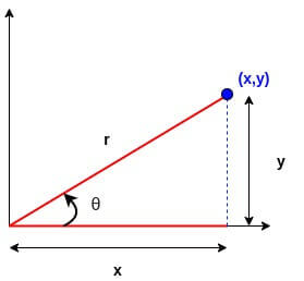
In this system, we denote the positions in a plane using a radius r (from the origin) and an angle θ (with the horizontal).
We can convert cartesian coordinates to polar coordinates and vice-versa using the following formulae
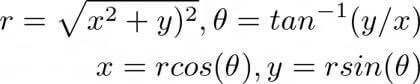
The following figure shows the two coordinate systems in the same plane, which will help you understand the relationship between them better.
Now that we understand the polar coordinate system and its relationship with the Cartesian system, and since we have already created a meshgrid of Cartesian coordinates,
Let us create a meshgrid of polar coordinates.
R = np.linspace(1,5,10)
THETA = np.linspace(0, np.pi, 45)
radii, thetas = np.meshgrid(R,THETA)
print("R:{}".format(R.shape))
print("THETA:{}".format(THETA.shape))
print("meshgrid radii:{}".format(radii.shape))
print("mehgrid thetas:{}".format(thetas.shape))
Output:
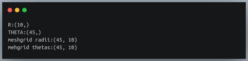
We have first defined the range for the radii. It’s ten equally spaced values from 1 to 5.
Then, we have defined the range for the angle, from 0 to π, or from 0° to 180°. We are considering 45 distinct values in this range.
Then, we create the meshgrid of these radii and angles.
As a result, we get two matrices, one each for the radii and the angles. Each of the two matrices is of the shape 45×10.
Let us now try visualizing these generated points on a polar coordinate plane using pyplot.
import matplotlib.pyplot as plt
ax = plt.subplot(111, polar=True)
ax.plot(thetas, radii, marker='.', ls='none')
plt.show()
Output:
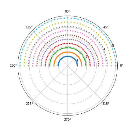
450 points are plotted in this figure representing the meshgrid created from 45 angles and 10 radii.
NumPy meshgrid with ‘matrix indexing’
We have so far observed that the np.meshgrid method returns the coordinates with Cartesian indexing
That means the first array represents the columns (X coordinates), and the second array the rows (Y coordinates).
However, if you consider the 2D arrays or matrices used in Computer Science, we access such arrays using ‘row first’ indexing,
i.e the first coordinate represents the rows, and the second, the column. Such indexing is called the ‘matrix indexing’.
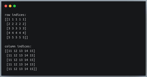
We can generate meshgrids with matrix indexing by assigning the string ‘ij’ to the parameter ‘indexing‘ of the np.meshgrid method.
i = np.array([1,2,3,4,5]) #rows
j = np.array([11, 12, 13, 14, 15]) #columns
ii, jj = np.meshgrid(i,j, indexing='ij')
print("row indices:\n{}\n".format(ii))
print("column indices:\n{}".format(jj))
Output:
If you look closely, these are the transpose of the arrays generated earlier using the default Cartesian (x, y) indexing.
Let us validate this observation.
print("ii equal to xx transposed ? ==>",np.all(ii == xx.T))
print("jj equal to yy transposed ? ==>",np.all(jj == yy.T))
Output:

Flip a NumPy meshgrid
Once we have x and y coordinates, we can flip the meshgrid vertically or horizontally, by manipulating the individual output arrays.
Let us first create a meshgrid of 150 values, and plot it so that we can visualize the flipping of the meshgrid.
X = np.linspace(1,15,15)
Y = np.linspace(20,30,10)
xx, yy = np.meshgrid(X,Y)
fig = plt.figure()
ax = fig.add_subplot(111)
ax.plot(xx, yy, ls="None", marker=".")
plt.show()
Output:
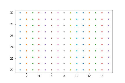
The figure contains 150 points in the meshgrid. Each column has points of the same color.
We can flip the meshgrid along the vertical axis by reversing the two coordinate arrays column-wise.
fig = plt.figure()
ax = fig.add_subplot(111)
ax.plot(xx[:,::-1], yy[:,::-1], ls="None", marker=".")
plt.show()
Output:
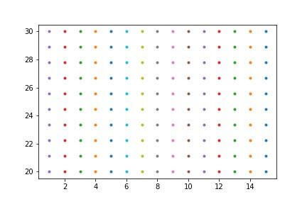
The meshgrid in this figure is flipped along the vertical axis from the previous figure.
This is denoted by the interchange of colors of points between the first and last columns, the second and second-to-last columns, and so on.
Creating Meshgrid with NumPy matrices
We have been creating meshgrids using 1-dimensional NumPy arrays.
But what happens if we pass 2 or more dimensional NumPy arrays as parameters for x and y?
We will use NumPy random seed so you can get the same random numbers on your computer.
np.random.seed(42)
a = np.random.randint(1,5, (2,2))
b = np.random.randint(6,10, (3,3))
print("a:\n{}\n".format(a))
print("b:\n{}".format(b))
xx, yy = np.meshgrid(a,b)
print("xx:\n{}".format(xx))
print("shape of xx:{}\n".format(xx.shape))
print("yy:\n{}".format(yy))
print("shape of yy:{}\n".format(yy.shape))
Output:
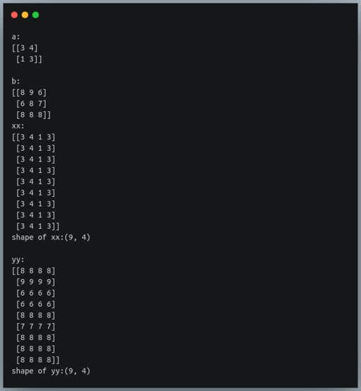
As is evident, irrespective of the shape of the input parameters, we get 2-dimensional NumPy arrays as output as long as the number of input arrays is two.
This is equivalent to flattening the input arrays before creating the meshgrid.
xx, yy = np.meshgrid(a.ravel(),b.ravel()) #passing flattened arrays
print("xx:\n{}".format(xx))
print("shape of xx:{}\n".format(xx.shape))
print("yy:\n{}".format(yy))
print("shape of yy:{}\n".format(yy.shape))
Output:
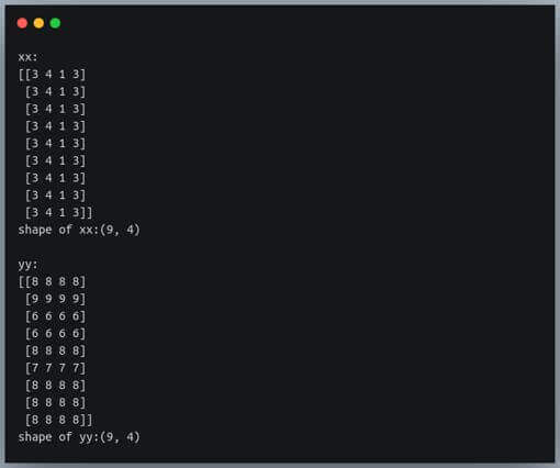
The output is identical to the one we got when we passed 2D arrays in their original shape to create the meshgrid.
Creating a 3-dimensional meshgrid
We have thus far only seen the construction of meshgrids in a 2D plane.
By supplying the x and y coordinate arrays, we get two output arrays, one each for the x and y coordinates in a 2D plane.
Let us now look at how we can generate a meshgrid in a 3D space, defined by 3 coordinates.
X = np.linspace(1,4,4)
Y = np.linspace(6,8, 3)
Z = np.linspace(12,15,4)
xx, yy, zz = np.meshgrid(X,Y,Z)
print(xx.shape, yy.shape, zz.shape)
Output:
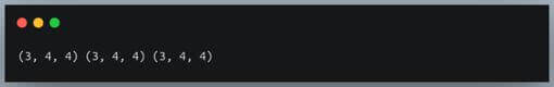
Now we are getting 3 output arrays, one each for the x, y and z coordinates in a 3D space.
Moreover, each of these three arrays is also 3-dimensional.
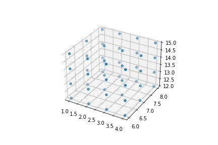
Let us visualize these coordinates on a 3d plot.
fig = plt.figure()
ax = fig.add_subplot(111, projection='3d')
ax.scatter(xx, yy, zz)
ax.set_zlim(12, 15)
plt.show()
Output:
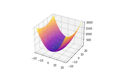
Creating a 3D surface plot using NumPy meshgrid
Let us now work out one of the applications of using np.meshgrid, which is creating a 3D plot.
We will first create a 2D meshgrid of x and y coordinates, and compute the third axis (z) values as a function of x and y.
from mpl_toolkits.mplot3d import Axes3D
X = np.linspace(-20,20,100)
Y = np.linspace(-20,20,100)
X, Y = np.meshgrid(X,Y)
Z = 4*xx**2 + yy**2
fig = plt.figure()
ax = fig.add_subplot(111, projection='3d')
ax.plot_surface(X, Y, Z, cmap="plasma", linewidth=0, antialiased=False, alpha=0.5)
plt.show()
Output:
Avoiding NumPy meshgrid memory error
When we assign values to a variable or perform any computation, these values are stored in our computer’s ‘temporary’ memory or RAM.
These memories come in a range of 8–32 GBs.
While creating meshgrids, we need to be careful not to create such a large meshgrid that would not fit in the memory.
For example, let us try creating a meshgrid of size 100000×100000 floating-point numbers.
X = np.random.randn(100000)
Y = np.random.randn(100000)
xx,yy =  np.meshgrid(X,Y)
Output:
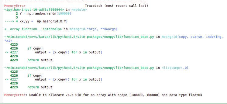
Here we are trying to generate a grid having 10 billion floating-point numbers.
If each floating-point number takes 8 bytes of memory, 10 billion such numbers would need about 74 GB of memory, which is not common even in modern personal computers.
Since the memory required to accommodate such a large meshgrid exceeds the available memory, we are getting this ‘MemoryError’.
Therefore, we must be cautious not to create too large a meshgrid, by either smoothening our data or choosing a smaller range for coordinates.
Note that even if the chosen size is large and within the limit of your memory, it may cause your computer to freeze if there’s no free memory left on the machine.
Conclusion
In this tutorial, we understood what are meshgrids and their various advantages.
We learned how to create a rectangular grid of coordinates using NumPy’s meshgrid method.
We also looked at the sparse representation of these meshgrids.
Then we learned how we can use the meshgrid method to generate a grid of polar coordinates.
We understood the two types of indexing when creating meshgrid, namely, the Cartesian (default) indexing and the matrix indexing.
After that, we looked at how we can flip a meshgrid. We also tried creating meshgrids by passing 2-dimensional arrays as input.
Then we generated 3D grids using 3 arrays, one each for x, y, and z dimensions.
We then looked at the application of the meshgrid method in creating 3D surface plots.
Finally, we looked at the problem of ‘Memory Error’ when creating meshgrids, and how to avoid them.
Machine Learning Engineer & Software Developer working on challenging problems in Computer Vision at IITK Research and Development center.
3+ years of coding experience in Python, 1+ years of experience in Data Science and Machine Learning.
Skills: C++, OpenCV, Pytorch, Darknet, Pandas, ReactJS, Django.