NumPy matrix multiplication (From Theory to Real-World Examples)
Matrix multiplication is a fundamental operation in linear algebra that takes a pair of matrices and produces another matrix.
In mathematical terms, given two matrices ( A ) and ( B ), the product ( AB ) is computed by taking the dot product of the rows of ( A ) with the columns of ( B ).
This tutorial aims to provide an in-depth understanding of matrix multiplication using NumPy,
- 1 Element-wise vs. Matrix Multiplication
- 2 Multiplication using np.dot
- 3 The np.matmul Function
- 4 The @ Operator
- 5 Comparing np.dot, np.matmul, and @
- 6 Multiplication with Scalars
- 7 In-place Multiplication with a Scalar
- 8 Time Complexity of np.dot, np.matmul, and @
- 9 Parallel Processing and GPU Acceleration
- 10 Type Errors
- 11 Real-World Example Using Matrix Multiplication
- 12 Resources
Element-wise vs. Matrix Multiplication
Element-wise multiplication, also known as the Hadamard product, multiplies the corresponding elements of two matrices of the same shape.
Example:
import numpy as np
A = np.array([[1, 2], [3, 4]])
B = np.array([[5, 6], [7, 8]])
result = A * B
print(result)
Output:
[[ 5, 12],
 [21, 32]]
Each element in the resulting matrix is the product of the corresponding elements in matrices ( A ) and ( B ):
- ( 1 X 5 = 5 )
- ( 2X 6 = 12 )
- ( 3 X 7 = 21 )
- ( 4 X 8 = 32 )
Matrix multiplication, on the other hand, requires that the number of columns in the first matrix is equal to the number of rows in the second matrix.
It’s a more complex operation that involves the dot product of rows and columns.
Using the same matrices ( A ) and ( B ), we get:
result = np.dot(A, B)
print(result)
Output:
[[19, 22],
 [43, 50]]
Multiplication using np.dot
The np.dot function in NumPy is one of the primary ways to perform matrix multiplication. It handles both two-dimensional arrays (matrices) and one-dimensional arrays (vectors).
Multiplying Matrices
Here’s an example using the np.dot function to multiply two matrices:
import numpy as np
A = np.array([[1, 2], [3, 4]])
B = np.array([[5, 6], [7, 8]])
result = np.dot(A, B)
print(result)
Output:
[[19, 22],
 [43, 50]]
The output is obtained by performing standard matrix multiplication, where the rows of the first matrix are multiplied with the corresponding columns of the second matrix.
Multiplying Vectors
np.dot can also be used to compute the dot product of two vectors:
v1 = np.array([3, 4])
v2 = np.array([5, 6])
result = np.dot(v1, v2)
print(result)
Output:
39
The output is the dot product of the vectors ( v1 ) and ( v2 ), computed as ( 3X 5 + 4X 6 = 39 ).
The np.matmul Function
Unlike np.dot, np.matmul is specifically designed for matrix multiplication and provides a more explicit way to perform this operation.
Here’s how to use np.matmul to multiply two matrices:
import numpy as np
A = np.array([[1, 2], [3, 4]])
B = np.array([[5, 6], [7, 8]])
result = np.matmul(A, B)
print(result)
Output:
[[19, 22],
 [43, 50]]
The output is identical to the result obtained with np.dot, as np.matmul also performs standard matrix multiplication.
Multi-dimensional arrays multiplication
np.matmul also handles multi-dimensional arrays and provides specific behavior for array broadcasting.
Example:
A = np.random.rand(2, 3, 4)
B = np.random.rand(2, 4, 3)
result = np.matmul(A, B)
print(result.shape)
Output:
(2, 3, 3)
In this case, np.matmul performs matrix multiplication over the last two dimensions of the input arrays and broadcasts over the remaining dimensions. The resulting shape is (2, 3, 3).
The @ Operator
In Python 3.5 and later versions, you can use the @ operator as a shorthand for matrix multiplication. This operator provides a clean and concise way to multiply matrices.
Here’s an example of how to use the @ operator to multiply two matrices:
import numpy as np
A = np.array([[1, 2], [3, 4]])
B = np.array([[5, 6], [7, 8]])
result = A @ B
print(result)
Output:
[[19, 22],
 [43, 50]]
The result is identical to that obtained with np.dot or np.matmul. The @ operator simplifies the code and makes the matrix multiplication operation visually clear.
The @ operator can also be used with higher-dimensional arrays, just like np.matmul, following the same broadcasting rules.
Comparing np.dot, np.matmul, and @
Understanding the differences and similarities between np.dot, np.matmul, and the @ operator can help you choose the right tool for your specific needs.
np.dot
- Can be used for both matrix multiplication and vector dot products.
- Handles two-dimensional arrays as general matrix multiplication.
- For higher-dimensional arrays, its behavior may differ from
np.matmul.
np.matmul
- Specifically designed for matrix multiplication.
- Provides consistent behavior across different dimensions.
- Handles broadcasting over the last two dimensions for multi-dimensional arrays.
@ Operator
- For Python 3.5 and above.
- Provides a clean and concise notation for matrix multiplication.
Multiplication with Scalars
In addition to multiplying matrices, you can multiply a matrix by a scalar (a single numerical value). This operation multiplies every element of the matrix by the scalar.
import numpy as np
A = np.array([[1, 2], [3, 4]])
scalar = 2
result = A * scalar
print(result)
Output:
[[2, 4],
 [6, 8]]
The output is obtained by multiplying every element in matrix ( A ) by the scalar value 2:
- ( 1X2 = 2 )
- ( 2X 2 = 4 )
- ( 3 X 2 = 6 )
- ( 4 X 2 = 8 )
In-place Multiplication with a Scalar
In-place multiplication with a scalar means modifying the original matrix by multiplying it with a scalar, without creating a new copy of the matrix.
This can be useful for memory efficiency, especially when dealing with large matrices.
You can use the *= operator to multiply a matrix with a scalar in place.
import numpy as np
A = np.array([[1, 2], [3, 4]])
scalar = 2
A *= scalar
print(A)
Output:
[[2 4]
[6 8]]
The matrix A is multiplied by 2 in-place, meaning that the original matrix A is modified without creating a new matrix.
You can also use numpy.multiply function with the out argument to achieve in-place multiplication.
A = np.array([[1, 2], [3, 4]])
scalar = 2
np.multiply(A, scalar, out=A) # In-place multiplication
print(A)
Output:
[[2 4]
[6 8]]
The np.multiply function with the out argument pointing to the original matrix A ensures that the multiplication is performed in-place.
Space complexity comparison
We can use the memory_profiler package to profile the memory usage of the scalar multiplication.
from memory_profiler import memory_usage

def inplace_multiplication(numbers, scalar):
    for i in range(len(numbers)):
        numbers[i] *= scalar

def multiplication_with_scalar(numbers, scalar):
    result = [num * scalar for num in numbers]

def main():
    numbers = [1, 2, 3, 4, 5] * 1000000
    scalar = 2
    mem_usage_inplace = memory_usage((inplace_multiplication, (numbers, scalar)))
    print(f'In-place multiplication memory used: {max(mem_usage_inplace) - min(mem_usage_inplace)} MiB')
    mem_usage_with_scalar = memory_usage((multiplication_with_scalar, (numbers, scalar)))
    print(f'Multiplication with scalar memory used: {max(mem_usage_with_scalar) - min(mem_usage_with_scalar)} MiB')
if __name__ == '__main__':
    main()
Output:
In-place multiplication memory used: 0.2265625 MiB
Multiplication with scalar memory used: 37.125 MiB
In-place multiplication is significantly lower in memory usage.
Time Complexity of np.dot, np.matmul, and @
Let’s measure the execution time for each method using the time module.
import numpy as np
import time
A = np.random.rand(5000, 5000)
B = np.random.rand(5000, 5000)

# Measuring time for np.dot
start_time = time.time()
result_dot = np.dot(A, B)
end_time = time.time()
print(f"np.dot execution time: {(end_time - start_time) :.2f} seconds")

# Measuring time for np.matmul
start_time = time.time()
result_matmul = np.matmul(A, B)
end_time = time.time()
print(f"np.matmul execution time: {(end_time - start_time) :.2f} seconds")

# Measuring time for @ operator
start_time = time.time()
result_at_operator = A @ B
end_time = time.time()
print(f"@ operator execution time: {(end_time - start_time) :.2f} seconds")
Output (example times; actual times may vary):
np.dot execution time: 1.13 seconds
np.matmul execution time: 1.18 seconds
@ operator execution time: 1.17 seconds
The execution times for np.dot, np.matmul, and the @ operator are reflecting the actual performance for these methods which is almost the same.
Parallel Processing and GPU Acceleration
Parallel processing and GPU (Graphics Processing Unit) acceleration can significantly speed up matrix multiplication, especially with large matrices.
NumPy itself does not offer direct GPU acceleration but can leverage libraries that do.
Libraries like CuPy provide a NumPy-compatible interface for GPU-accelerated computations.
First, install CuPy which corresponds to your CUDA version. Then, you can perform GPU-accelerated matrix multiplication as follows:
import cupy as cp
A_gpu = cp.random.rand(1000, 1000)
B_gpu = cp.random.rand(1000, 1000)

# Matrix multiplication on the GPU
result_gpu = A_gpu @ B_gpu
By simply replacing NumPy with CuPy, you can execute the same code on a GPU.
This can lead to a substantial performance increase for large-scale matrix multiplication.
Considerations
- GPU acceleration is most effective for large matrices where the parallelism of the GPU can be fully utilized.
- Data transfer between CPU and GPU can introduce overhead, especially for small matrices.
- Not all NumPy functions are supported in GPU-accelerated libraries, so compatibility should be checked.
Type Errors
In matrix multiplication, understanding the data types of the matrices involved is essential.
Mixing integer and float matrices can lead to unexpected results or type errors. Here’s how to handle them:
Implicit Type Conversion
When multiplying an integer matrix with a float matrix, NumPy performs implicit type conversion, converting the integer matrix to float.
import numpy as np
A = np.array([[1, 2], [3, 4]], dtype=int)
B = np.array([[1.5, 2.5], [3.5, 4.5]], dtype=float)
result = A @ B
print(result.dtype)
Output:
float64
Here, the integer matrix A is implicitly converted to float before multiplication, and the result is a float matrix.
Explicit Type Conversion
Explicitly converting matrices to a common data type can prevent unexpected behavior.
Example:
A = A.astype(float)  # Explicitly converting A to float
result = A @ B
By explicitly converting A to float, you ensure that the multiplication proceeds as expected, with no surprises related to data types.
Real-World Example Using Matrix Multiplication
Scaling a 2D Object in Computer Graphics
Suppose you have a 2D triangle defined by its vertices, and you want to scale it.
1. Define the Object
Start by defining the coordinates of the triangle’s vertices as a matrix.
import numpy as np

# Vertices of the triangle
triangle_vertices = np.array([
    [0, 0],
    [4, 0],
    [2, 3]
])
Here, the vertices are augmented with an additional dimension to handle the translation using homogeneous coordinates.
2. Define the Scaling Matrix
Create a scaling matrix that scales by 2 in the x-direction and 3 in the y-direction.
scale_x = 2
scale_y = 3
scaling_matrix = np.array([
    [scale_x, 0],
    [0, scale_y]
])
3. Perform the Scaling
Multiply the vertices by the scaling matrix to scale the triangle.
scaled_triangle_vertices = triangle_vertices.dot(scaling_matrix)
print(scaled_triangle_vertices)
Output:
array([[0, 0],
       [8, 0],
       [4, 9]]))
The triangle has been scaled by a factor of 2 in the x-direction and 3 in the y-direction.
Let’s draw the scaled coordinates to draw the scaled object in matplotlib:
import matplotlib.pyplot as plt
def plot_triangle(vertices, color, label):
    plt.plot(*vertices.T, color=color, label=label) # Plot the edges
    plt.scatter(*vertices.T, color=color) # Plot the vertices
    plt.fill(vertices[:, 0], vertices[:, 1], alpha=0.1, color=color) # Fill the triangle

# Plot the original triangle
plot_triangle(triangle_vertices, color='blue', label='Original Triangle')

# Plot the scaled triangle
plot_triangle(scaled_triangle_vertices, color='red', label='Scaled Triangle')

# Add labels and legend
plt.xlabel('X')
plt.ylabel('Y')
plt.legend()
plt.grid(True)
plt.axis('equal') # Equal scaling ensures that the plot is not distorted
plt.title('Scaling Transformation of a 2D Triangle')
plt.show()
Output:
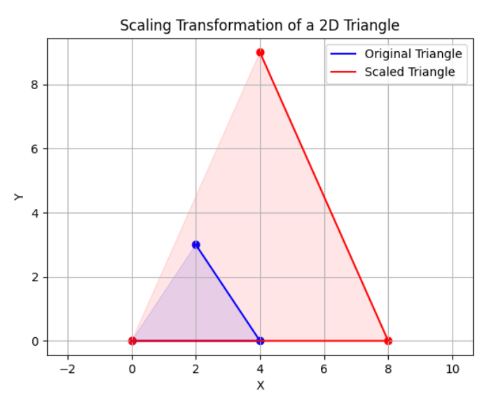
Image Rotation
First, the image is loaded in color, and the color scheme is converted from BGR to RGB since OpenCV reads images in BGR by default. The necessary libraries are also imported.
import numpy as np
from scipy.ndimage import affine_transform
import cv2
import matplotlib.pyplot as plt
image = cv2.imread("image.jpg")
image = cv2.cvtColor(image, cv2.COLOR_BGR2RGB) # Convert from BGR to RGB
Combine Transformation using matrix multiplication
Then we define the rotation angle and create the corresponding rotation matrix.
Additionally, we compute the transformation matrix to shift the center of rotation to the center of the image.
Matrix multiplication is then used to combine these transformations into the full_transform matrix.
angle_degrees = 60
angle_radians = np.radians(angle_degrees)
rotation_matrix = np.array([[np.cos(angle_radians), -np.sin(angle_radians), 0],
                            [np.sin(angle_radians), np.cos(angle_radians), 0],
                            [0, 0, 1]])
height, width, _ = image.shape
center_x, center_y = width // 2, height // 2
transform_matrix = np.array([[1, 0, -center_x],
                             [0, 1, -center_y],
                             [0, 0, 1]])

# Combine the shift and rotation using matrix multiplication
full_transform = np.dot(np.linalg.inv(transform_matrix), rotation_matrix)
full_transform = np.dot(full_transform, transform_matrix)
In the final step, the rotation is applied to the image by using the affine_transform function from the SciPy library.
This is done separately for each color channel to handle the 3D nature of the image. Finally, the rotated image is displayed using Matplotlib.
rotated_image = np.zeros_like(image)
for channel in range(image.shape[2]):
    rotated_image[..., channel] = affine_transform(image[..., channel], full_transform[:2, :2], offset=(full_transform[0, 2], full_transform[1, 2]))
plt.imshow(rotated_image)
plt.title("Rotated Image")
plt.axis("off")
plt.show()
Output:

Resources
https://numpy.org/doc/stable/reference/generated/numpy.dot.html
https://numpy.org/doc/stable/reference/generated/numpy.matmul.html
Mokhtar is the founder of LikeGeeks.com. He is a seasoned technologist and accomplished author, with expertise in Linux system administration and Python development. Since 2010, Mokhtar has built an impressive career, transitioning from system administration to Python development in 2015. His work spans large corporations to freelance clients around the globe. Alongside his technical work, Mokhtar has authored some insightful books in his field. Known for his innovative solutions, meticulous attention to detail, and high-quality work, Mokhtar continually seeks new challenges within the dynamic field of technology.