Profiling in Python (Detect CPU & memory bottlenecks)
Have you been working with datasets in your code that have huge chunks of data, and as soon as you execute your code, you find that the code is taking an eternity to produce the final output?
Well, that can be frustrating! You have probably used the correct syntax, and the logic is also right. Yet the code consumes an enormous amount of RAM and takes too long to execute.
This is when you should think of optimizing your code to utilize the CPU resources better. Finding the cause and locating the place of its occurrence is extremely important to determine an optimal solution.
In this case, what would be your approach? Will you experiment with your code using a hit and trial method to locate the places in your code that consume maximum resources?
That is one way of doing it, but certainly not the best way. Python leverages us with amazing tools known as profilers, which make life easy for us by detecting the exact areas within your code responsible for the poor performance of the overall code.
Simply put, profiling refers to the detailed accounting of the different resources your code uses and how the code is using these resources.
In this tutorial, we will dive deep into numerous profilers and learn how to visualize the bottlenecks in our code that will enable us to identify issues to optimize and enhance the performance of our code.
What is profiling?
If a program is consuming too much RAM or taking too long to execute, then it becomes necessary to find out the reason behind such hindrances in the overall performance of your code.
This means you need to identify which part of your code is hampering the performance.
You can fix the issue by optimizing the part of code that you believe is the major reason behind the bottleneck. But more often than not, you might end up fixing the wrong section of your code in an attempt to guess the location of your problem wildly.
Rather than simply wandering in search of the epicenter of the issue, you should opt for a deterministic approach that will help you to locate the exact resources causing the hindrance in performance.
This is where profiling comes into the picture.
Profiling allows you to locate the bottleneck in your code with minimum effort and allows you to optimize your code for maximum performance gains.
The best part about profiling is that any resource that can be measured (not just the CPU time and memory) can be profiled.
For example, you can also measure network bandwidth and disk I/O. In this tutorial, we will focus on optimizing CPU time and memory usage with the help of Python profilers.
Hence, without further delay, let us dive into the numerous methods offered by Python to perform deterministic profiling of Python programs.
Using time module
Python provides a plethora of options for measuring the CPU time of your code. The simplest among these is the time module. Let’s consider that our code takes an enormous amount of time to execute.
This is where you can use timers to calculate the execution time of your code and keep optimizing it on the fly. Timers are extremely easy to implement and can be used almost anywhere within the code.
Example: In the following snippet, we will look at a very simple piece of code that measures the time taken by the code for executing a simple function.
import time
def linear_search(a, x):
   for i in range(len(a)):
       if a[i] == x:
           return i
   return -1
start = time.time()
print(linear_search([10, 20, 30, 40, 50, 60, 70, 80, 90, 100], 50))
stop = time.time()
print("Time Consumed: {} secs".format(stop - start))
Output: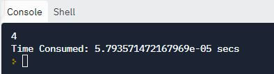
Explanation: In the above code, we implemented a linear search upon a given list and searched a specific number within this list using a function.
The time() method of the time module allowed us to keep a track of the time required to execute this piece of code by tracking the time elapsed to execute the entire linear_search() function.
The difference between the start time and stop time is the actual taken for the function to compute the output in this case.
Thus, it gave us a clear idea about the time taken to search an element in the list using our linear_search function.
Discussion: Given the length of the list, this was a super-fast search mechanism; hence it was not a big issue. However, think of a huge list consisting of thousands of numbers.
Well, in that case, this search technique might not prove to be the best algorithm in terms of time consumed by the code.
So, here’s another method that helps to search the same element but takes less time, thereby allowing us to optimize our code.
We will once again check the time elapsed with the help of our time.time() function to compare the time taken by the two codes.
import time
def binary_search(a, x):
   low = 0
   high = len(a) - 1
   mid = 0
   while low <= high:
       mid = (high + low) // 2
       if a[mid] < x:
           low = mid + 1
       elif a[mid] > x:
           high = mid - 1
       else:
           return mid
   return -1
start = time.time()
print(binary_search([10, 20, 30, 40, 50, 60, 70, 80, 90, 100], 50))
stop = time.time()
print("Time Consumed: {} secs".format(stop - start))
Output: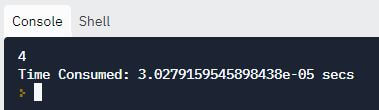
When we compare the two outputs, it is evident that binary search consumes lesser time than the linear search method.
Thus, the time.time() function enabled us to track the time taken by our code to search a particular element from the list, and that allowed us to improve the performance of our code with the help of the optimal search algorithm.
Using cProfile
Though the time module helped us to track the time taken by the code to reach the final output, it did not provide us with too much information.
We had to identify the optimal solution by comparing the time elapsed by each algorithm through manual analysis of our code.
But, there will be instances in your code wherein you will need the help of certain other parameters to identify which section of your code caused the maximum delay.
This is when you can use the cProfile module. cProfile is a built-in module in Python that is commonly used to perform profiling.
Not only does it provide the total time taken by the code to execute, but it also displays the time taken by each step.
This, in turn, allows us to compare and locate the parts of code which actually need to be optimized.
Another benefit of using cProfile is that if the code has numerous function calls, it will display the number of times each function has been called.
This can prove to be instrumental in optimizing different sections of your code.
Note: cProfile facilitates us with the cProfile.run(statement, filename=None, sort=-1) function that allows us to execute profiling upon our code.
Within the statement argument, you can pass the code or the function name that you want to profile. If you wish to save the output to a certain file, then you can pass the name of the file to the filename argument.
The sort argument is used to specify the order in which the output has to be printed. Let’s have a look at an example that utilizes the cProfile module to display CPU usage statistics.
import cProfile
def build():
   arr = []
   for a in range(0, 1000000):
       arr.append(a)
def deploy():
   print('Array deployed!')
def main():
   build()
   deploy()
if __name__ == '__main__':
   cProfile.run('main()')
Output: 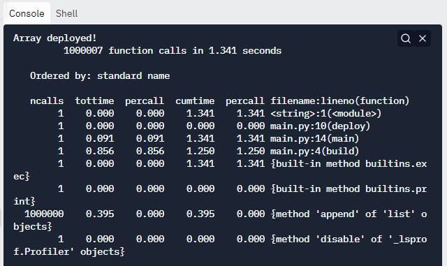
Explanation:
-
- After the output is displayed, the next information that cProfile displays is the number of function calls that took place within the code and the total time taken to perform those function calls.
- The next piece of information is “Ordered by: standard name”, which denotes that the string in the rightmost column was used to sort the output.
The column headings of the table include the following information:
-
- ncalls: represents the number of calls.
- tottime: denotes the total time taken by a function. It excludes the time taken by calls made to sub-functions.
- percall: (tottime)/(ncalls)
- cumtime: represents the total time taken by a function as well as the time taken by subfunctions called by the parent function.
- percall: (cumtime)/( primitive calls)
- filename:lineno(function): gives the respective data of every function.
A slight improvement to this code can be made by printing the output within the build() method itself. This will reduce a single function call and help us to slightly improve the execution time of the code.
This can be better visualized with the help of nested functions. Hence, let us visualize the significance of profiling with respect to nested functions.
Profiling nested functions
Let’s implement profiling on a nested function, i.e., a function that calls another function to visualize how cProfile helps us to optimize our code.
import cProfile
def build():
   arr = []
   for a in range(0, 1000000):
       if check_even(a):
           arr.append(a)
def check_even(x):
   if x % 2 == 0:
       return x
   else:
       return None
if __name__ == '__main__':
   cProfile.run('build()')
Output: 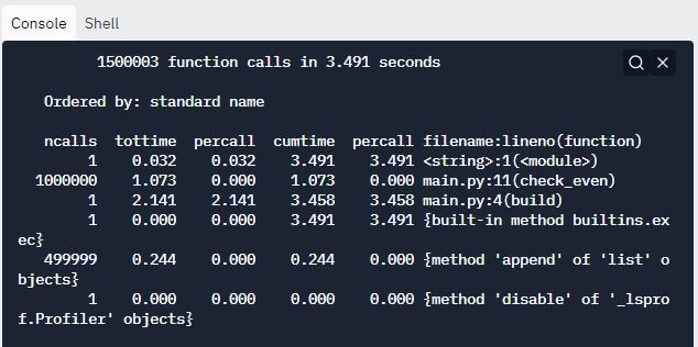
The above cProfile report clearly suggests that the check_even method has been called 1000000 times. This is unnecessary and is responsible for hampering the performance of our code.
Thus, we can optimize our code by eliminating this function call and performing the required check within the loop itself, as shown in the snippet below.
import cProfile
def build():
   arr = []
   for a in range(0, 1000000):
       if a % 2 == 0:
           arr.append(a)
if __name__ == '__main__':
   cProfile.run('build()')
Output: 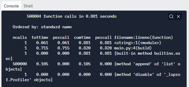
We have successfully eliminated the unnecessary function calls in our code, thereby significantly enhancing the overall performance of our code.
Visualize profiling using GProf2Dot
One of the best ways to identify bottlenecks is to visualize the performance metrics. GProf2Dot is a very efficient tool to visualize the output generated by our profiler.
Example: Assume that we are profiling the following snippet:
import cProfile
import pstats
def build():
    arr = []
    for a in range(0, 1000000):
        arr.append(a)
if __name__ == '__main__':
    profiler = cProfile.Profile()
    profiler.enable()
    build()
    profiler.disable()
    stats=pstats.Stats(profiler).sort_stats(-1)
    stats.print_stats()
    stats.dump_stats('output.pstats')
Installation
You must use the pip to install gprof2dot:
pip install gprof2dot
NOTE: To visualize the graph, you must ensure that Graphviz is installed. You can download it from this link: https://graphviz.org/download/
Generating the pstats file
Once you have finished installing the required libraries, you can profile your script to generate the pstats file using the following command:
python -m cProfile -o output.pstats demo.py
Visualizing the stats
Execute the following command in your terminal where the pstats output file is located:
gprof2dot -f pstats output.pstats | "C:\Program Files\Graphviz\bin\dot.exe" -Tpng -o output.png
That’s all. You will find a PNG file generated within the same directory which looks something like this:
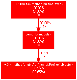
NOTE: You might encounter peculiar errors while creating the graph from the pstats file in Windows. Hence it is a good idea to use the entire path of the dot file as shown above.
Visualize profiling using snakeviz
Another incredible way of visualizing the pstats output is to use the snakeviz tool, which gives you a clear picture of how the resources are being utilized. You can install it using the pip installer: “pip install snakeviz.”
Once you have installed the snakeviz tool, you need to execute your code from the command line and generate the .prof file. Once the .prof file is generated, you must execute the following command to visualize the statistics on your browser:
snakeviz demo.prof
Example: In the following code, we will visualize how the nested function consumes resources.
def build():
   arr = []
   for a in range(0, 1000000):
       if check_even(a):
           arr.append(a)
def check_even(x):
   if x % 2 == 0:
       return x
   else:
       return None
build()
To visualize the output using snakeviz, use the following command on your terminal.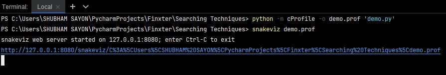
There are two visualization styles exhibited by Snakeviz: icicle and sunburst. The default style is Icicle, wherein the time consumed by different sections of the code is represented by the width of rectangles.
Whereas in the case of the sunburst view, it is represented by the angular extent of an arc. Let’s have a look at the icicle and sunburst views for the above code.
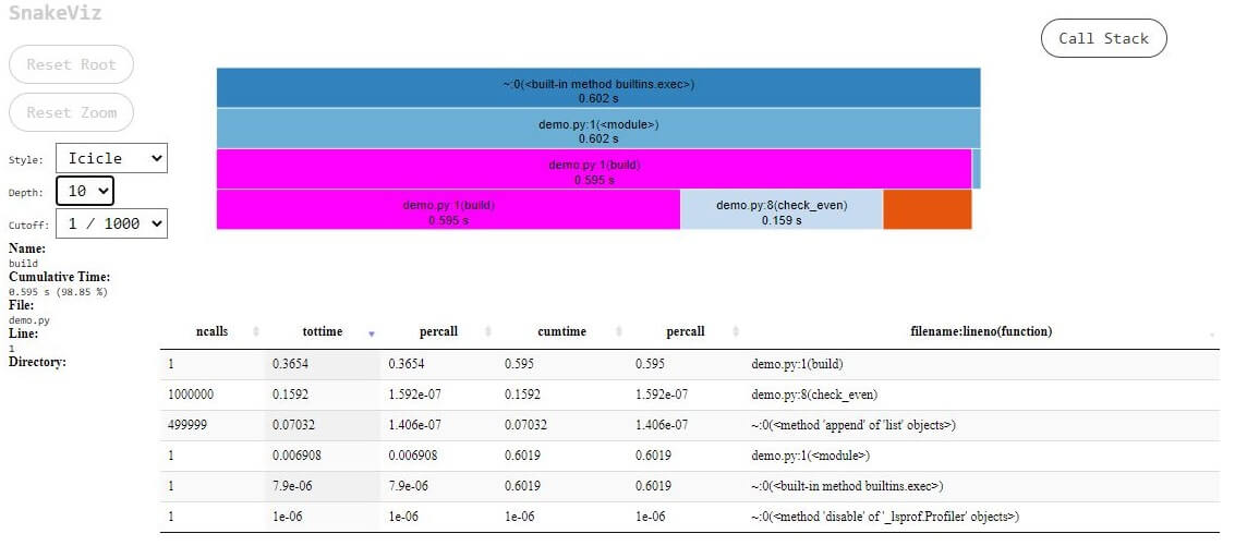
Fig.1 – SnakeViz Icicle View
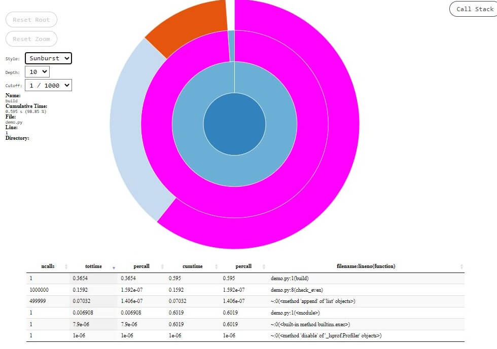
Fig.2 – SnakeViz Sunburst View
Python line profiler
CProfiler allows us to detect how much time is consumed by each function within the code, but it does not provide information about the time taken by each line within the code.
Sometimes, profiling only at the function call level does not solve the problem, as it causes confusion when a certain function is called from different parts of the code.
For example, the function might perform well under call#1, but it depletes performance at call#2. This cannot be identified through function-level profiling.
Thus, Python provides a library known as line_profiler, which enables us to perform line-by-line profiling of our code.
In the following example, we will visualize how to use a line_profiler from the shell. The given snippet has a main() function that calls three other functions.
Every function called by the main function generates 100000 random numbers and prints their average.
The sleep() method within each function ensures that each function takes different amounts of time to complete the operation.
To be able to visualize the output generated by the line profiler, we have used the @profile decorator for each function in the script.
import time
import random
def method_1():
   time.sleep(10)
   a = [random.randint(1, 100) for i in range(100000)]
   res = sum(a) / len(a)
   return res
def method_2():
   time.sleep(5)
   a = [random.randint(1, 100) for i in range(100000)]
   res = sum(a) / len(a)
   return res
def method_3():
   time.sleep(3)
   a = [random.randint(1, 100) for i in range(100000)]
   res = sum(a) / len(a)
   return res
def main_func():
   print(method_1())
   print(method_2())
   print(method_3())
main_func()
We can use the following command to execute and profile the above snippet:
kernprof -l demo_line_profiler.py
NOTE: You must install the line profiler before you can perform line-by-line profiling with its help. To install it, use the following command:
pip install line-profiler
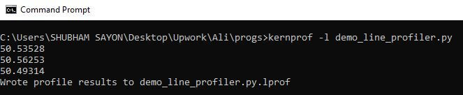
The kernprof command generates the script_name.lprof file once it completes profiling the entire script. The .lprof file gets created and resides in the same project folder.
Now, execute the following command in the terminal to visualize the output:
python -m line_profiler demo_line_profiler.py.lprof
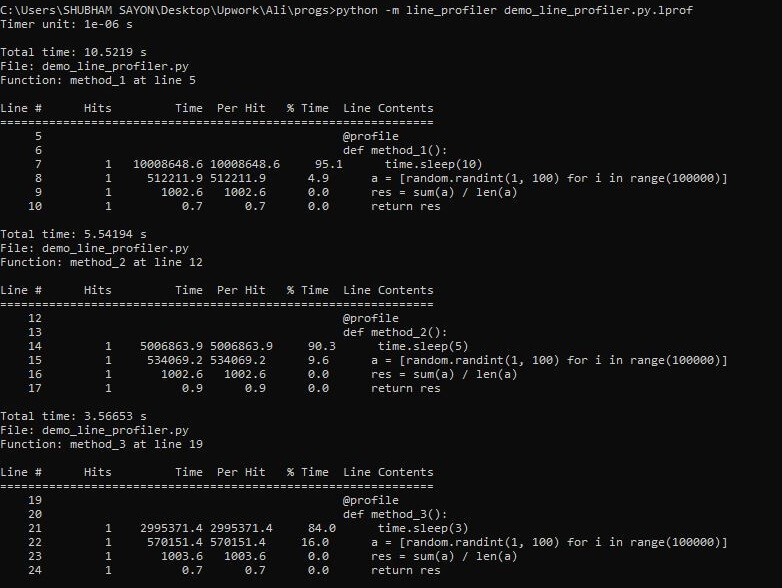
It is evident from the above output that the line profiler has generated a table for each function. Let’s understand the meaning of each column in the table.
1. Hits represent the number of times the particular line was hit inside that function.
2. Time represents the time taken by that particular line to perform all the hits.
3. Per Hit denotes the total time taken for each function call to complete that line.
4. % Time represents the percentage of time taken by the line when compared to the total time taken by the function.
5. Line Content represents a line of the function.
Using Pyinstrument
Pyinstrument is a statistical Python profiler that is quite similar to cProfile. But it has certain advantages over the cProfile profiler.
1. It does not record the whole function call stack all at once. Instead, it records the call stack every 1 ms. This, in turn, helps to reduce profiling overhead.
2. It is more concise than cProfile as it only shows the major functions that are responsible for taking maximum time. Therefore, it eliminates the faster segments and avoids profiling noise.
Another great advantage of using the Pyinstrument is that the output can be visualized in many ways, including HTML. You can even have a look at the full timeline of calls.
However, a major disadvantage of using Pyinstrument is that it is not very efficient in dealing with codes that run in multiple threads.
Example: In the following script, we will generate a couple of random numbers and find their sum. Then we will append the sum to a list and return it.
NOTE: You must install Pyinstrument using the following command:
pip install pyinstrument
import random
def addition(x, y):
   return x + y
def sum_list():
   res = []
   for i in range(1000000):
       num_1 = random.randint(1, 100)
       num_2 = random.randint(1, 100)
       add = addition(num_1, num_2)
       res.append(add)
   return res
if __name__ == "__main__":
   o = sum_list()
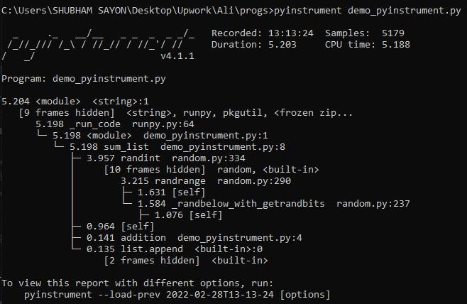
We can execute the code to visualize the pyinstrument output using the following command:
pyinstrument demo_pyinstrument.py
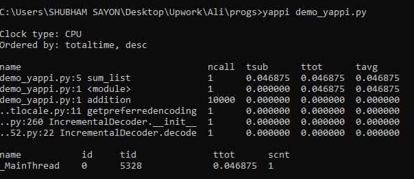
Using Yappi
Yet another Python profiler, abbreviated as Yappi, is a Python profiler that has been designed in C. It supports the profiling of multithreaded codes. It performs function-level profiling.
It also allows us to format the profiling output in numerous formats, like callgrind and pstat.
Yappi leverages us the ability to decide whether we want to profile the CPU time or the wall time.
CPU time is the total time taken by the code during which it used the CPU, whereas the walltime is the time during which the code ran, starting from the first line to the last line.
Yappi stores the output as a stat object that allows us to filter the profiling results and sort them. We can invoke, start, stop and generate profiling reports with the help of Yappi.
Example: In the following code, we have a function that iterates through 100000 numbers and doubles each number before appending it to a list. We will then profile it using Yappi.
def addition(x, y):
   return x+y
def sum_list():
   res = []
   for i in range(10000):
       out = addition(i, i)
       res.append(out)
   return res
if __name__ == "__main__":
   o = sum_list()
Output:
Using Palanteer
Palanteer is another profiling tool that can be used to profile Python as well as C++ code.
Hence, it is a powerful tool to have in your arsenal if you deal with Python code that wraps C++ libraries and you want a deep insight into the components of your application.
Palanteer uses a GUI app that displays the results, which makes it extremely useful to track and visualize the stats on the go.
Palanteer tracks almost every performance parameter, starting from function calls to OS-level memory allocations.
However, the problem with palanteer is that you have to build it from scratch, i.e., from the source. It does not have precompiled binaries yet.
Python memory-profiler
We have gone through a world of profilers and examples that demonstrate how we can profile our code to measure the time taken for its execution.
There are other factors as well, like memory usage, which dictate the performance of our code.
Thus, to visualize the memory usage by different resources within our code, Python provides us with a memory profiler that measures the memory usage. To use the memory profiler, you must install it using pip:
pip install -U memory_profiler
Just like the line profiler, the memory profiler is used to track line-by-line memory usage. You have to decorate each function with the @profile decorator to view the usage statistics and then run the script using the following command:
python -m memory_profiler script_name.py
In the following code, we will store values within the range of 100000 in a list and then visualize the memory usage with the help of the memory profiler.
@profile
def foo():
   li = []
   for i in range(100000):
       li.append(i)
foo()
Output: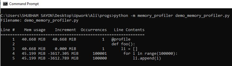
Python Pympler
In many cases, it is required to monitor memory usage with the help of an object. This is where a Python library known as pympler becomes handy to meet the requirements.
It provides us with a list of modules that monitor memory usage in various ways.
In this tutorial, we will have a look at the assizeof module that accepts one or more objects as an input and returns the size of each object in bytes.
NOTE: You must install pympler before you use it:
pip install Pympler
Example: In the following code, we will create a couple of lists and store values within two different ranges and then use the asizeof module of the pympler library to find out the size occupied by each list object.
from pympler import asizeof
li_1 = [x for x in range(100)]
li_2 = [y for y in range(100000)]
print("Space occupied by li_1 : %d bytes"%asizeof.asizeof(li_1))
print("Space occupied by li_2 : %d bytes"%asizeof.asizeof(li_2))
print("Space occupied by li_1 + li_2: %d bytes"%asizeof.asizeof(li_1,li_2))
Output: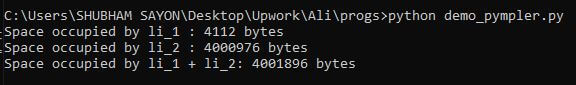
Mokhtar is the founder of LikeGeeks.com. He is a seasoned technologist and accomplished author, with expertise in Linux system administration and Python development. Since 2010, Mokhtar has built an impressive career, transitioning from system administration to Python development in 2015. His work spans large corporations to freelance clients around the globe. Alongside his technical work, Mokhtar has authored some insightful books in his field. Known for his innovative solutions, meticulous attention to detail, and high-quality work, Mokhtar continually seeks new challenges within the dynamic field of technology.