Visualize NumPy Complex Arrays with 3D Plots in Python

Complex numbers are essential in various fields, including signal processing and quantum mechanics.

In this tutorial, you’ll learn how to visualize NumPy complex arrays using 3D plots in Python.

 

 

Understand the Structure of Complex Arrays

Complex arrays in NumPy consist of two main components: real and imaginary parts.

These components can be represented in different forms, such as magnitude and phase.

To create a complex array, you can use NumPy’s complex function:

import numpy as np
x = np.linspace(-5, 5, 100)
y = np.linspace(-5, 5, 100)
X, Y = np.meshgrid(x, y)
Z = X + 1j * Y
print(Z.shape)
print(Z[0, 0])

Output:

(100, 100)
(-5-5j)

This code creates a 100×100 complex array where each element’s real part comes from X and the imaginary part from Y.

The shape of Z is (100, 100), and the first element is -5-5j which represents the complex number at the bottom-left corner of the grid.

 

Extract Real and Imaginary Parts

You can extract the real and imaginary parts of a complex array using NumPy real and imag functions:

real_part = np.real(Z)
imag_part = np.imag(Z)
print(real_part[0, 0])
print(imag_part[0, 0])

Output:

-5.0
-5.0

The real_part and imag_part arrays contain the real and imaginary components of Z, respectively.

In this case, both the real and imaginary parts of the first element are -5.0.

 

Compute Magnitude and Phase

To compute the magnitude and phase of complex numbers, you can use NumPy abs and angle functions:

magnitude = np.abs(Z)
phase = np.angle(Z)
print(magnitude[0, 0])
print(phase[0, 0])

Output:

7.0710678118654755
-2.356194490192345

The magnitude of the first element is approximately 7.07 (sqrt(5^2 + 5^2)), and its phase is about -2.36 radians (-3π/4).

 

Plot Real and Imaginary Parts in 3D

To create 3D surface plots of the real and imaginary parts, you can use Matplotlib plot_surface function:

import matplotlib.pyplot as plt
fig = plt.figure(figsize=(12, 5))
ax1 = fig.add_subplot(121, projection='3d')
ax1.plot_surface(X, Y, real_part, cmap='viridis')
ax1.set_title('Real Part')
ax2 = fig.add_subplot(122, projection='3d')
ax2.plot_surface(X, Y, imag_part, cmap='plasma')
ax2.set_title('Imaginary Part')
plt.tight_layout()
plt.show()

Output:

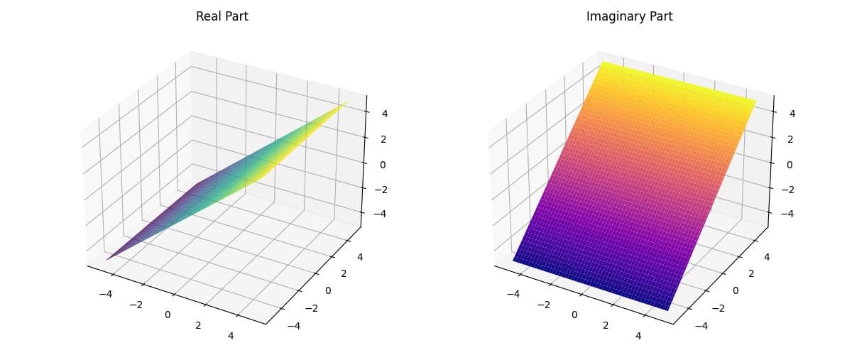
This code creates two 3D surface plots: one for the real part and another for the imaginary part of the complex array.

The real part shows a plane tilted along the x-axis, while the imaginary part shows a plane tilted along the y-axis.

 

Visualize Magnitude of Complex Arrays

To visualize the magnitude of complex arrays, you can create a 3D surface plot:

fig = plt.figure(figsize=(10, 8))
ax = fig.add_subplot(111, projection='3d')
surf = ax.plot_surface(X, Y, magnitude, cmap='viridis')
ax.set_title('Magnitude of Complex Array')
fig.colorbar(surf)
plt.show()

Output:

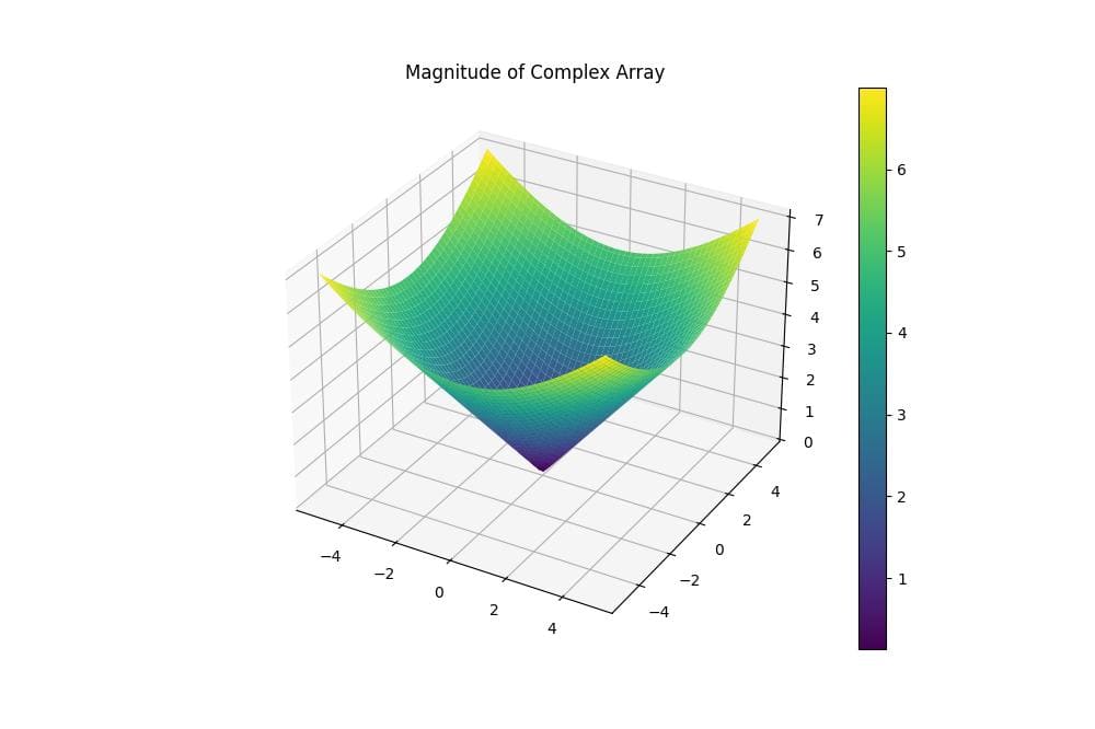
This plot displays the magnitude of the complex array as a 3D surface.

The resulting plot shows a cone-like shape, with the magnitude increasing as you move away from the origin.

 

Visualize Phase of Complex Arrays

To represent the phase of complex arrays in 3D, you can use a similar way:

fig = plt.figure(figsize=(10, 8))
ax = fig.add_subplot(111, projection='3d')
surf = ax.plot_surface(X, Y, phase, cmap='cool')
ax.set_title('Phase of Complex Array')
fig.colorbar(surf)
plt.show()

Output:

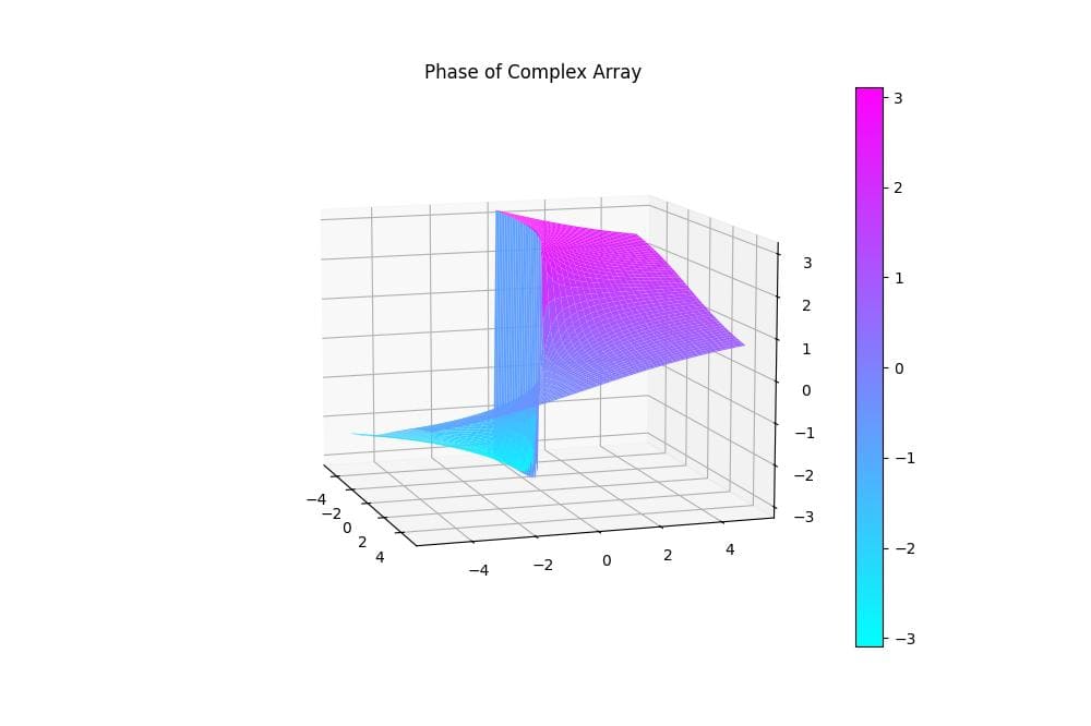
This plot shows the phase of the complex array as a 3D surface.

The resulting plot displays a twisted plane, with colors representing different phase values.

 

Combine Magnitude and Phase in a Single Plot

To combine magnitude and phase information in a single plot, you can use the magnitude for the height and the phase for the color:

fig = plt.figure(figsize=(10, 8))
ax = fig.add_subplot(111, projection='3d')
surf = ax.plot_surface(X, Y, magnitude, facecolors=plt.cm.hsv(phase / (2 * np.pi)))
ax.set_title('Magnitude and Phase of Complex Array')
cbar = fig.colorbar(surf, ax=ax, label='Phase', orientation='vertical')
cbar.set_ticks([-np.pi, -np.pi/2, 0, np.pi/2, np.pi])
cbar.set_ticklabels([r'$-\pi$', r'$-\pi/2$', '0', r'$\pi/2$', r'$\pi$'])
plt.show()

Output:

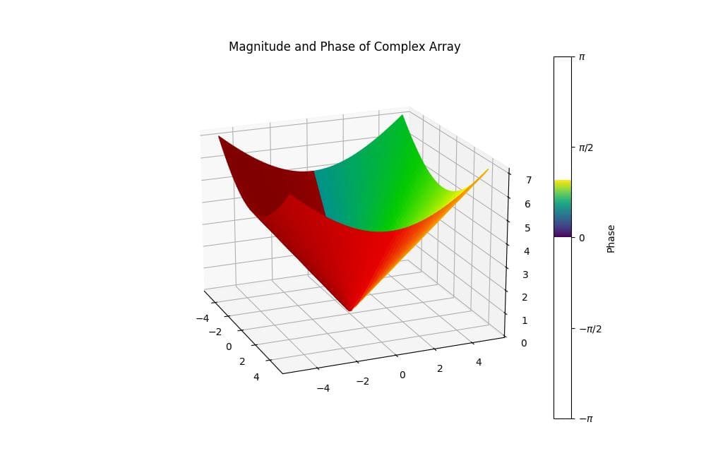
This plot combines the magnitude and phase information of the complex array.

The height of the surface represents the magnitude, while the colors represent the phase.

We set custom ticks and labels for the colorbar to show the phase range from -π to π.