Draw Multiple 3D Plots on The Same Figure in Python

In this tutorial, you’ll learn how to create multiple 3D plots on the same figure using the Python Matplotlib library.

You’ll explore various methods to combine different types of 3D plots, manage their visibility, and handle intersections.

 

 

Using ax.plot3D() Multiple Times

To create multiple line plots in 3D space, you can use the ax.plot3D() function multiple times on the same axes:

import numpy as np
import matplotlib.pyplot as plt
t = np.linspace(0, 10, 100)
x1, y1, z1 = np.cos(t), np.sin(t), t
x2, y2, z2 = np.cos(t) * t, np.sin(t) * t, t
fig = plt.figure(figsize=(10, 8))
ax = fig.add_subplot(111, projection='3d')
ax.plot3D(x1, y1, z1, 'b-', label='Helix')
ax.plot3D(x2, y2, z2, 'r-', label='Spiral')
ax.set_xlabel('X')
ax.set_ylabel('Y')
ax.set_zlabel('Z')
ax.legend()
plt.show()

Output:

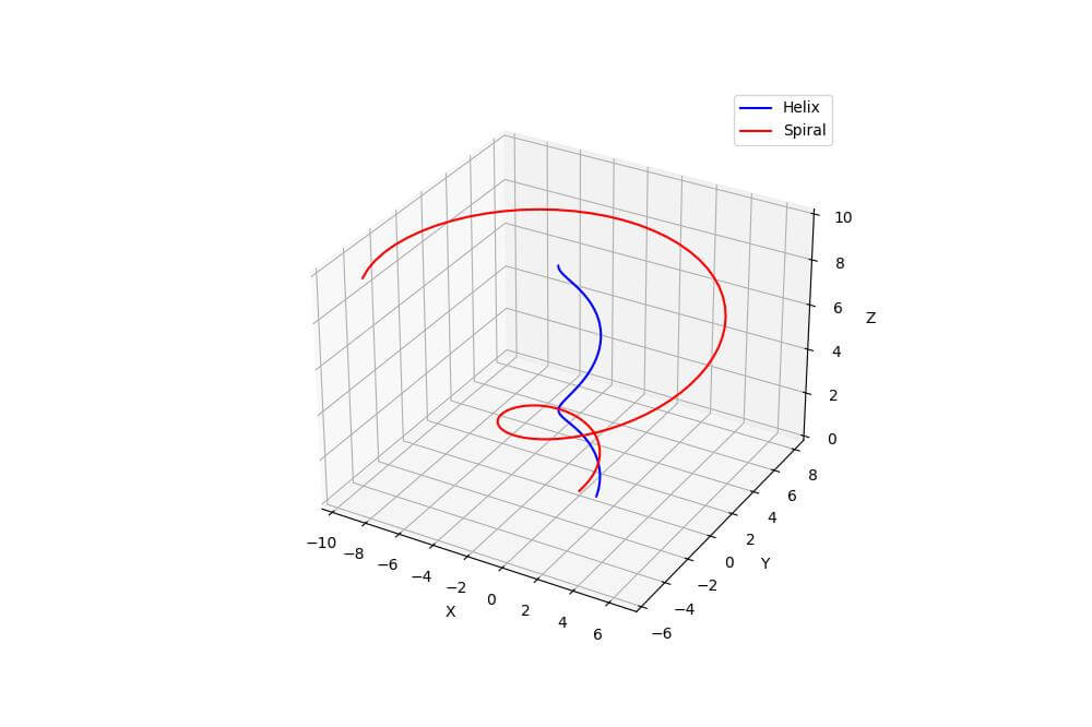
This code creates two 3D lines: a helix and a spiral.

The ax.plot3D() function is called twice, once for each line, with different data and colors.

 

Using ax.scatter3D() for Multiple Datasets

You can use ax.scatter3D() to plot multiple sets of points in 3D space:

import numpy as np
import matplotlib.pyplot as plt
np.random.seed(42)
n_points = 100
x1, y1, z1 = np.random.rand(3, n_points)
x2, y2, z2 = np.random.rand(3, n_points) + 0.5
fig = plt.figure(figsize=(10, 8))
ax = fig.add_subplot(111, projection='3d')
ax.scatter3D(x1, y1, z1, c='b', marker='o', label='Dataset 1')
ax.scatter3D(x2, y2, z2, c='r', marker='^', label='Dataset 2')
ax.set_xlabel('X')
ax.set_ylabel('Y')
ax.set_zlabel('Z')
ax.legend()
plt.show()

Output:

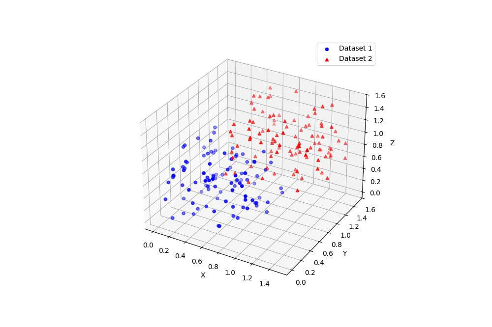
This code creates two sets of random 3D points and plots them using different colors and markers.

The resulting scatter plot allows you to visualize the distribution and relationship between the two datasets in 3D space.

 

Combine Different Plot Types

You can combine different types of 3D plots, such as surface and scatter plots, on the same axes:

import numpy as np
import matplotlib.pyplot as plt
x = np.linspace(-5, 5, 50)
y = np.linspace(-5, 5, 50)
X, Y = np.meshgrid(x, y)
Z = np.sin(np.sqrt(X**2 + Y**2))
n_points = 100
x_scatter = np.random.uniform(-5, 5, n_points)
y_scatter = np.random.uniform(-5, 5, n_points)
z_scatter = np.sin(np.sqrt(x_scatter**2 + y_scatter**2)) + np.random.normal(0, 0.1, n_points)
fig = plt.figure(figsize=(12, 9))
ax = fig.add_subplot(111, projection='3d')

# Plot surface
surf = ax.plot_surface(X, Y, Z, cmap='viridis', alpha=0.8)

# Plot scatter points
ax.scatter3D(x_scatter, y_scatter, z_scatter, c='r', s=50)
ax.set_xlabel('X')
ax.set_ylabel('Y')
ax.set_zlabel('Z')
plt.colorbar(surf, shrink=0.5, aspect=5)
plt.show()

Output:

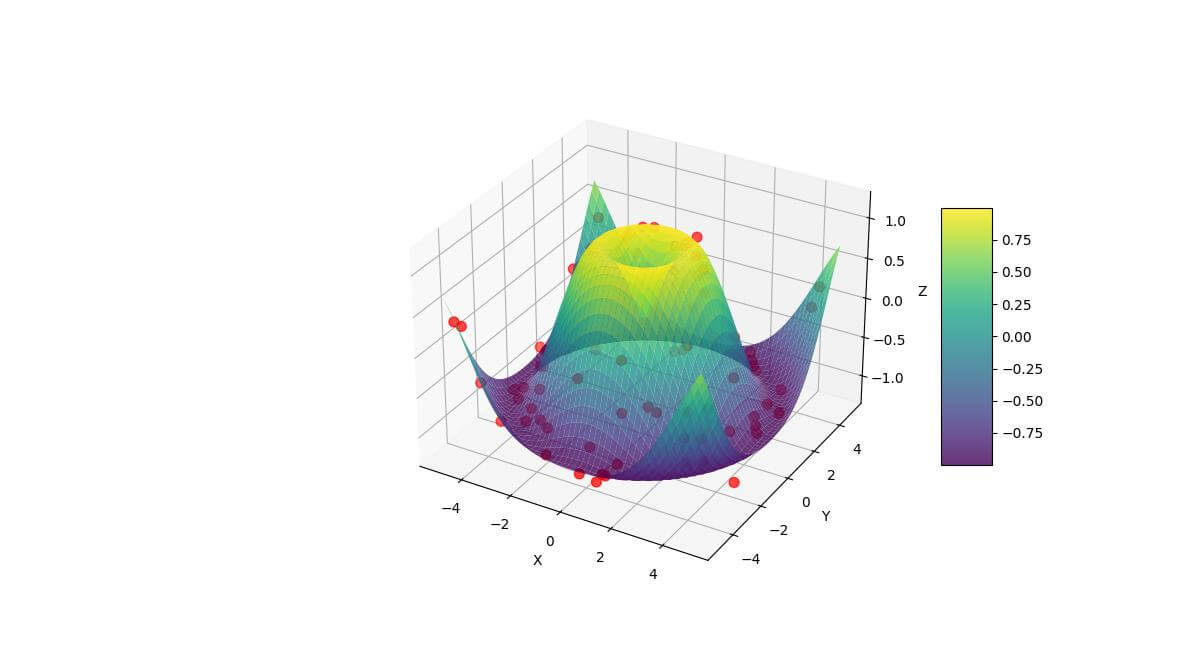
The surface plot uses a color map to represent the Z values, while the scattered points are shown in red.

This combination allows you to visualize both the overall trend of the data and individual data points.

 

Using ax.contour3D() for Multiple Contour Plots

You can create multiple 3D contour plots on the same axes using ax.contour3D() or ax.contourf3D():

import numpy as np
import matplotlib.pyplot as plt

# Create data for two contour plots
x = np.linspace(-5, 5, 50)
y = np.linspace(-5, 5, 50)
X, Y = np.meshgrid(x, y)
Z1 = np.sin(np.sqrt(X**2 + Y**2))
Z2 = np.cos(np.sqrt(X**2 + Y**2))
fig = plt.figure(figsize=(12, 9))
ax = fig.add_subplot(111, projection='3d')

# Plot filled contours for the first function
contourf1 = ax.contourf3D(X, Y, Z1, 50, cmap='viridis', alpha=0.5)

# Plot line contours for the second function
contour2 = ax.contour3D(X, Y, Z2, 20, cmap='plasma')
ax.set_xlabel('X')
ax.set_ylabel('Y')
ax.set_zlabel('Z')
plt.colorbar(contourf1, shrink=0.5, aspect=5, label='Function 1')
plt.colorbar(contour2, shrink=0.5, aspect=5, label='Function 2')
plt.show()

Output:

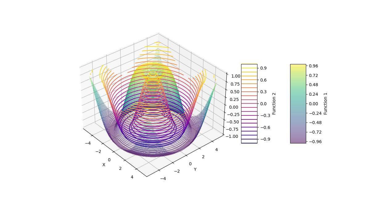
This code creates two 3D contour plots: a filled contour plot for a sine function and a line contour plot for a cosine function.

The filled contour plot uses transparency to allow visibility of the line contours behind it.

 

Plot Visibility and Layering

To control the visibility and layering of multiple 3D plots, you can adjust the order of plotting and use the zorder parameter:

import numpy as np
import matplotlib.pyplot as plt
from matplotlib.lines import Line2D
x = np.linspace(-5, 5, 50)
y = np.linspace(-5, 5, 50)
X, Y = np.meshgrid(x, y)
Z = np.sin(np.sqrt(X**2 + Y**2))

# Create scatter points
n_points = 100
x_scatter = np.random.uniform(-5, 5, n_points)
y_scatter = np.random.uniform(-5, 5, n_points)
z_scatter = np.sin(np.sqrt(x_scatter**2 + y_scatter**2)) + np.random.normal(0, 0.1, n_points)

# Create the figure and 3D axis
fig = plt.figure(figsize=(12, 9))
ax = fig.add_subplot(111, projection='3d')

# Plot surface with lower zorder
surf = ax.plot_surface(X, Y, Z, cmap='viridis', alpha=0.7, zorder=1)

# Plot scatter points with higher zorder
scatter = ax.scatter3D(x_scatter, y_scatter, z_scatter, c='r', s=50, zorder=2)
ax.set_xlabel('X')
ax.set_ylabel('Y')
ax.set_zlabel('Z')
plt.colorbar(surf, shrink=0.5, aspect=5)

# Create custom legend
custom_lines = [
  Line2D([0], [0], linestyle="none", c='r', marker='o'),
  Line2D([0], [0], linestyle="none", c='#1f77b4', marker='s')  # Use a specific color from viridis
]
ax.legend(custom_lines, ['Scatter Points', 'Surface'], numpoints=1)
plt.show()

Output:

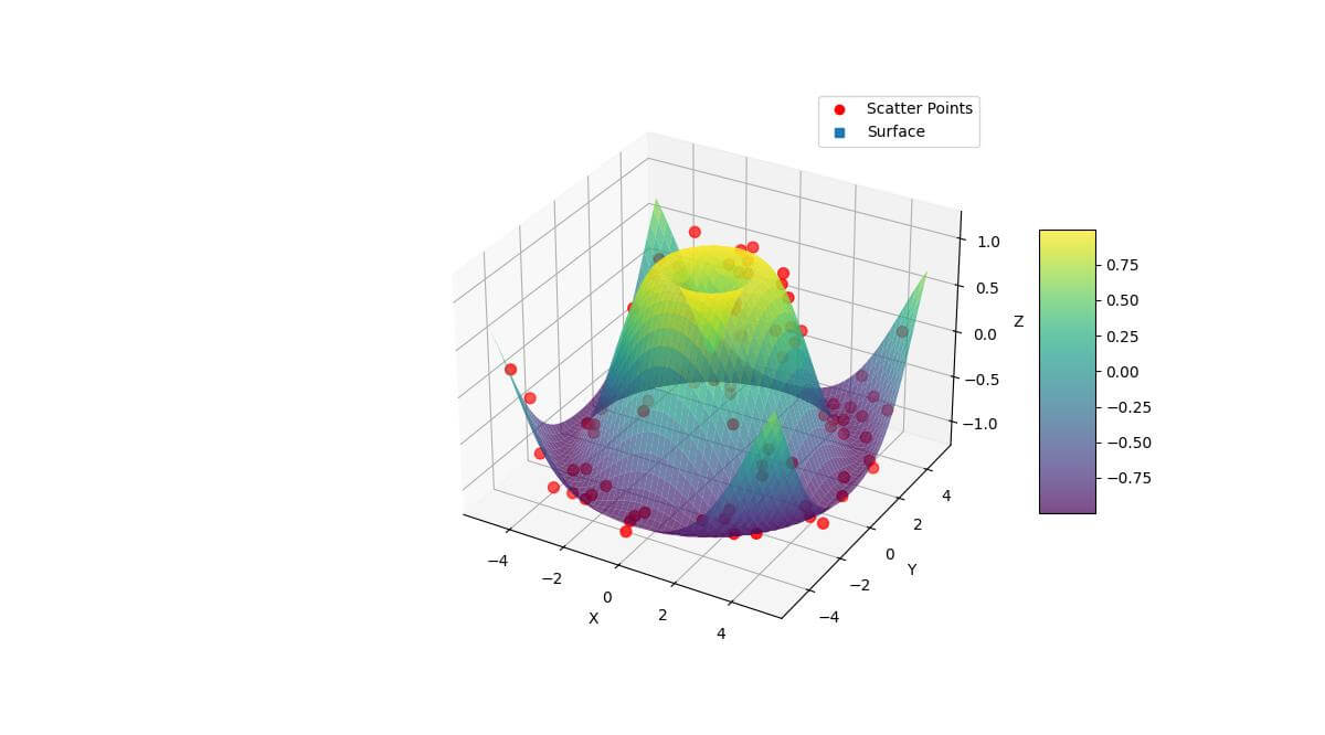
The surface plot is rendered first with a lower zorder value, while the scatter plot is rendered on top with a higher zorder.

This ensures that the scatter points are always visible above the surface.

 

Plot Intersections and Overlaps:

To handle intersections and overlaps between multiple 3D plots, you can use clipping planes:

import numpy as np
import matplotlib.pyplot as plt
x = np.linspace(-5, 5, 100)
y = np.linspace(-5, 5, 100)
X, Y = np.meshgrid(x, y)
Z1 = 2 * X + Y
Z2 = -X + 3 * Y
fig = plt.figure(figsize=(12, 9))
ax = fig.add_subplot(111, projection='3d')

# Plot the first plane
surf1 = ax.plot_surface(X, Y, Z1, cmap='viridis', alpha=0.7)

# Plot the second plane with a clipping plane
surf2 = ax.plot_surface(X, Y, Z2, cmap='plasma', alpha=0.7)

# Set up clipping plane
ax.set_xlim(-5, 5)
ax.set_ylim(-5, 5)
ax.set_zlim(-15, 15)

# Add a plane to show the intersection
xx, yy = np.meshgrid([-5, 5], [-5, 5])
zz = np.zeros_like(xx)
ax.plot_surface(xx, yy, zz, alpha=0.3, color='gray')
ax.set_xlabel('X')
ax.set_ylabel('Y')
ax.set_zlabel('Z')
plt.colorbar(surf1, shrink=0.5, aspect=5, label='Plane 1')
plt.colorbar(surf2, shrink=0.5, aspect=5, label='Plane 2')
plt.show()

Output:

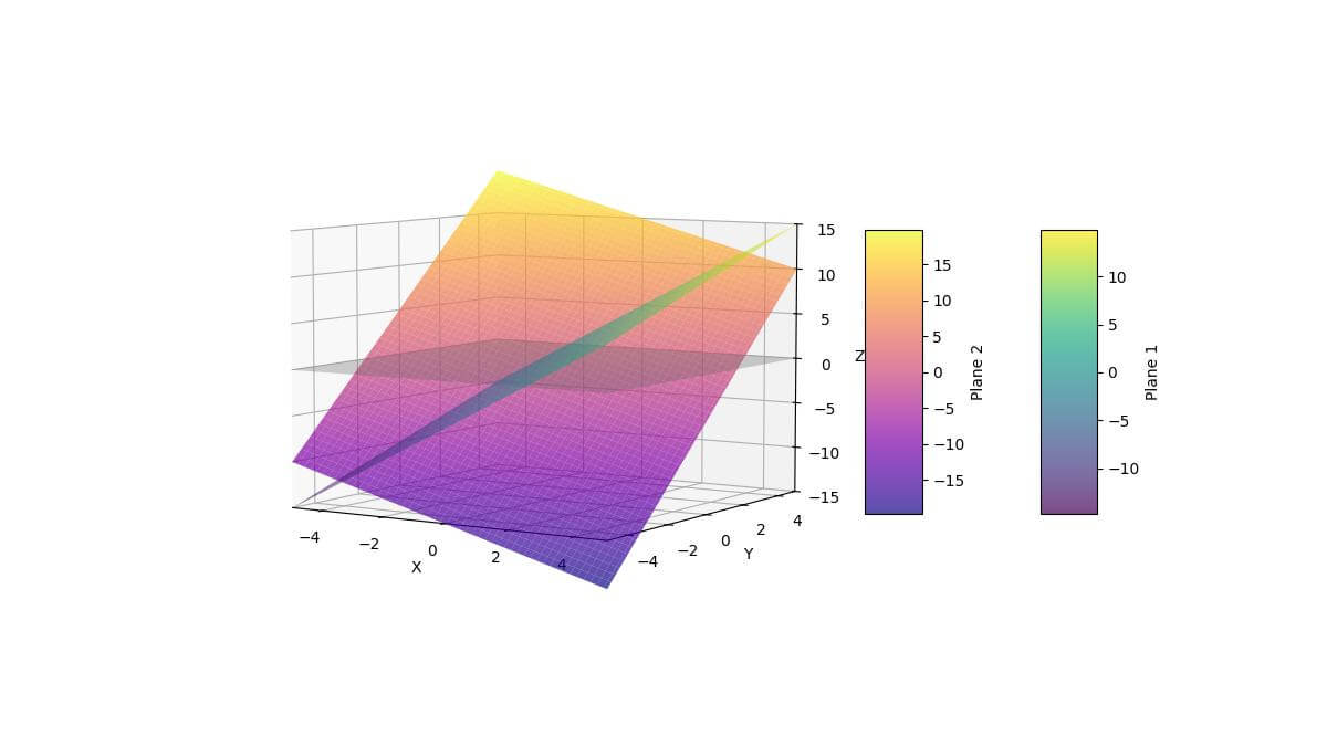
The clipping plane is represented by a semi-transparent gray surface at z=0.