Implement Low Pass Filter Using NumPy

In this tutorial, you’ll learn how to implement low-pass filters using NumPy in Python.

These filters are useful in reducing noise, smoothing data, and extracting meaningful information from signals in various fields.

You’ll learn about different types of filters, including Finite Impulse Response (FIR) filters and Fast Fourier Transform (FFT)-based filters.

 

 

FIR Filter – Finite Impulse Response

FIR filters are crucial in digital signal processing for filtering signals without introducing phase distortion.

First, let’s import the necessary libraries and define a function to create our FIR filter:

import numpy as np
import matplotlib.pyplot as plt

def create_fir_filter(num_taps, cutoff_frequency, sampling_rate):
    # Normalized cutoff frequency
    normalized_cutoff = 2 * cutoff_frequency / sampling_rate

    # Create an array of tap indices
    indices = np.arange(-num_taps // 2, num_taps // 2 + 1)

    # Calculate the sinc filter
    sinc_filter = np.sinc(normalized_cutoff * indices)

    # Apply a window function (Hann window)
    window = np.hanning(len(sinc_filter))
    fir_filter = sinc_filter * window
    return fir_filter

num_taps = 101
cutoff_frequency = 10
sampling_rate = 100
filter_coefficients = create_fir_filter(num_taps, cutoff_frequency, sampling_rate)
plt.plot(filter_coefficients)
plt.title('FIR Filter Coefficients')
plt.xlabel('Samples')
plt.ylabel('Amplitude')
plt.grid(True)
plt.show()

Output:

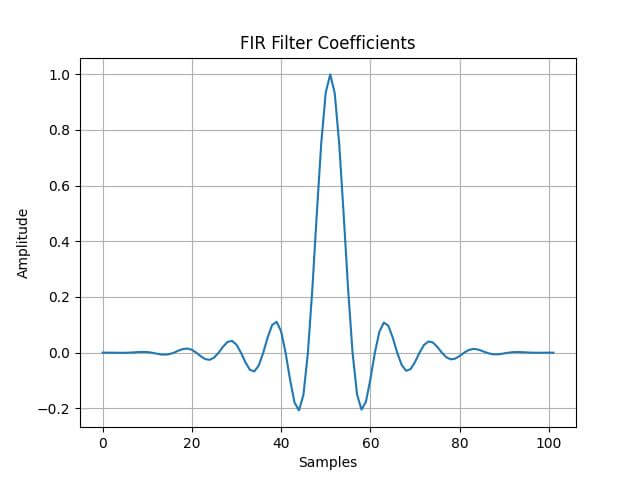
This plot visualizes the FIR filter coefficients. The filter is designed using a sinc function, which is the ideal low-pass filter in the frequency domain.

The windowing (Hann window in this case) smoothens the edges of the sinc function, reducing ripple in the frequency response and minimizing the effect of spectral leakage.

 

Using FFT Filter

The idea is to transform the signal into the frequency domain using FFT, apply a filter function (like a rectangular window), and then convert it back to the time domain using the inverse FFT.

Let’s start by taking the FFT of a signal, applying a rectangular window in the frequency domain, and then performing an inverse FFT:

def fft_filter(data, cutoff_frequency, sampling_rate):
    fft_data = np.fft.fft(data)
    frequencies = np.fft.fftfreq(len(data), d=1/sampling_rate)

    # Create a rectangular window (filter) in the frequency domain
    filter_mask = np.abs(frequencies) < cutoff_frequency

    # Apply the filter
    filtered_fft_data = fft_data * filter_mask

    # Perform inverse FFT
    filtered_data = np.fft.ifft(filtered_fft_data)
    return filtered_data.real

# Sample data
data = np.cos(2 * np.pi * 0.05 * np.arange(1000)) + np.random.randn(1000) * 0.1  # Signal with noise

# Filter parameters
cutoff_frequency = 0.1
sampling_rate = 1.0
filtered_data_fft = fft_filter(data, cutoff_frequency, sampling_rate)
plt.plot(data, label='Original Data')
plt.plot(filtered_data_fft, label='Filtered Data - FFT')
plt.title('FFT Filter Application')
plt.xlabel('Sample Number')
plt.ylabel('Amplitude')
plt.legend()
plt.grid(True)
plt.show()

Output:

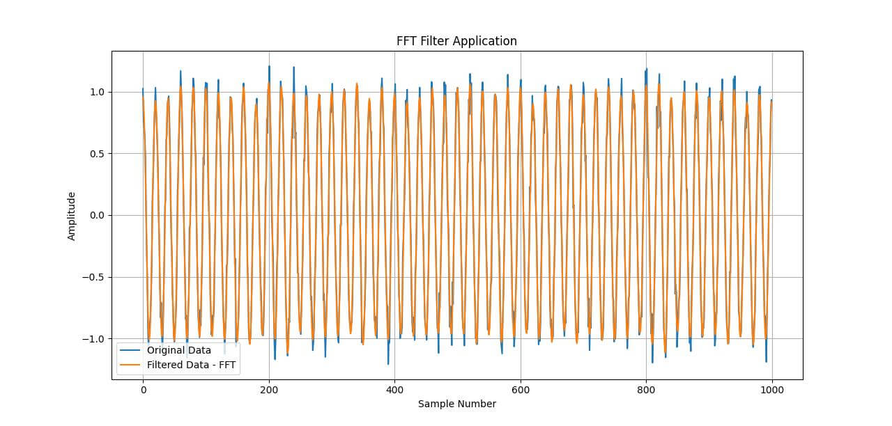
The rectangular window in the frequency domain successfully attenuates the higher frequency components, resulting in a cleaner signal.

FFT filters are useful for complex filtering tasks where traditional FIR and IIR filters might not be as effective.

 

Using numpy.convolve

Convolution is a fundamental concept in signal processing, and it’s useful for implementing filters.

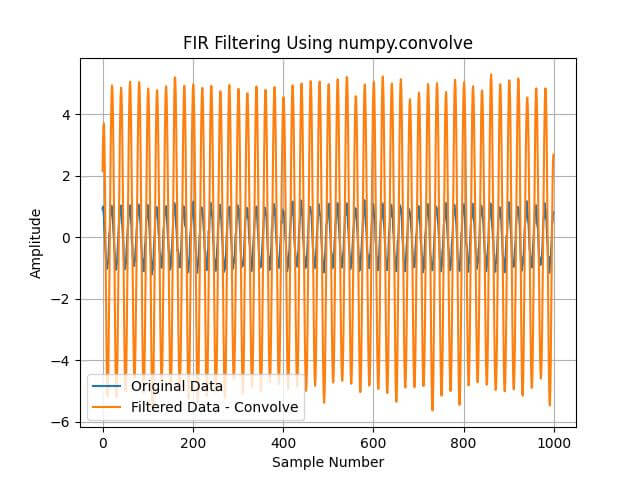
The FIR filter created earlier can be applied to a signal using the numpy.convolve method, which combines the filter coefficients with the signal.

def apply_fir_filter(signal, filter_coefficients):
    # Convolve the signal with the filter coefficients
    filtered_signal = np.convolve(signal, filter_coefficients, mode='same')
    return filtered_signal
data = np.cos(2 * np.pi * 0.05 * np.arange(1000)) + np.random.randn(1000) * 0.1  # Signal with noise

# Apply FIR filter using convolution
filtered_data_convolve = apply_fir_filter(data, filter_coefficients)

plt.plot(data, label='Original Data')
plt.plot(filtered_data_convolve, label='Filtered Data - Convolve')
plt.title('FIR Filtering Using numpy.convolve')
plt.xlabel('Sample Number')
plt.ylabel('Amplitude')
plt.legend()
plt.grid(True)
plt.show()

Output:

 

Practical Application (Blurring Images)

First, we’ll use the FIR filter to blur an image. Blurring is done by applying a low-pass filter, which removes high-frequency components (like edges and noise) from the image.

from PIL import Image
import numpy as np
from scipy.signal import convolve2d
image = Image.open('example.jpg')
image = image.convert('L')  # Convert to grayscale
image_data = np.array(image)

# Create a 2D FIR filter (average filter)
kernel_size = 15
fir_filter_2d = np.ones((kernel_size, kernel_size)) / kernel_size**2
blurred_image_data = convolve2d(image_data, fir_filter_2d, mode='same', boundary='wrap')
blurred_image = Image.fromarray(blurred_image_data)
blurred_image.show()

Original Image:

Output:

The code loads an image, converts it to grayscale, and then applies a 2D FIR filter.

The filter is a simple average filter, which blurs the image by averaging pixel values in the neighborhood defined by the filter size.