Mastering Colormaps in Python 3D Plotting

Colormaps are essential tools for visualizing data in 3D plots. They help you represent additional dimensions of information through color variations.

In this tutorial, you’ll learn how to use and manipulate colormaps in matplotlib to create better 3D visualizations.

 

 

Using Colormaps from External Libraries

You can use colormaps from external libraries like Seaborn to enhance your 3D plots.

import numpy as np
import matplotlib.pyplot as plt
from mpl_toolkits.mplot3d import Axes3D
import seaborn as sns
x = np.linspace(-5, 5, 100)
y = np.linspace(-5, 5, 100)
X, Y = np.meshgrid(x, y)
Z = np.sin(np.sqrt(X**2 + Y**2))

# Create the 3D plot using a Seaborn colormap
fig = plt.figure(figsize=(10, 8))
ax = fig.add_subplot(111, projection='3d')
surf = ax.plot_surface(X, Y, Z, cmap=sns.color_palette("rocket", as_cmap=True))
fig.colorbar(surf)
plt.show()

Output:

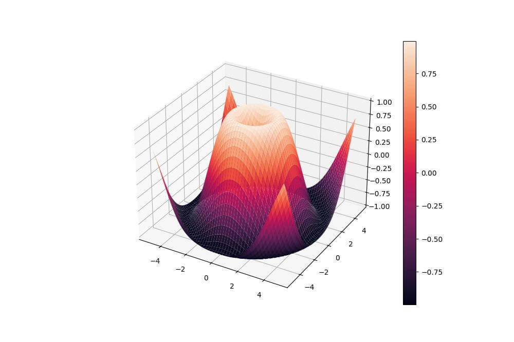
This code uses Seaborn “rocket” colormap to create a 3D surface plot.

 

Discrete Colormaps

You can create discrete colormaps for categorical data visualization.

import numpy as np
import matplotlib.pyplot as plt
from mpl_toolkits.mplot3d import Axes3D
from matplotlib.colors import BoundaryNorm, ListedColormap
x = np.linspace(-5, 5, 100)
y = np.linspace(-5, 5, 100)
X, Y = np.meshgrid(x, y)
Z = np.sin(np.sqrt(X**2 + Y**2))

# Create a discrete colormap
n_bins = 5
cmap = plt.get_cmap('viridis', n_bins)
norm = BoundaryNorm(np.linspace(-1, 1, n_bins + 1), n_bins)
fig = plt.figure(figsize=(10, 8))
ax = fig.add_subplot(111, projection='3d')
surf = ax.plot_surface(X, Y, Z, cmap=cmap, norm=norm)
fig.colorbar(surf, ticks=np.linspace(-1, 1, n_bins))
plt.show()

Output:

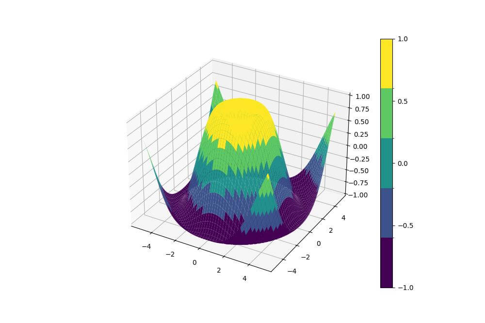
The BoundaryNorm is used to define the boundaries between these levels.

The colors change abruptly at specific thresholds.

 

Blending Multiple Colormaps

You can create complex visualizations by blending multiple colormaps.

import numpy as np
import matplotlib.pyplot as plt
from mpl_toolkits.mplot3d import Axes3D
from matplotlib.colors import LinearSegmentedColormap
x = np.linspace(-5, 5, 100)
y = np.linspace(-5, 5, 100)
X, Y = np.meshgrid(x, y)
Z = np.sin(np.sqrt(X**2 + Y**2))

# Create a custom blended colormap
cmap1 = plt.get_cmap('viridis')
cmap2 = plt.get_cmap('plasma')
colors1 = cmap1(np.linspace(0., 1, 128))
colors2 = cmap2(np.linspace(0., 1, 128))
colors = np.vstack((colors1, colors2))
blended_cmap = LinearSegmentedColormap.from_list('blended', colors)
fig = plt.figure(figsize=(10, 8))
ax = fig.add_subplot(111, projection='3d')
surf = ax.plot_surface(X, Y, Z, cmap=blended_cmap)
fig.colorbar(surf)
plt.show()

Output:

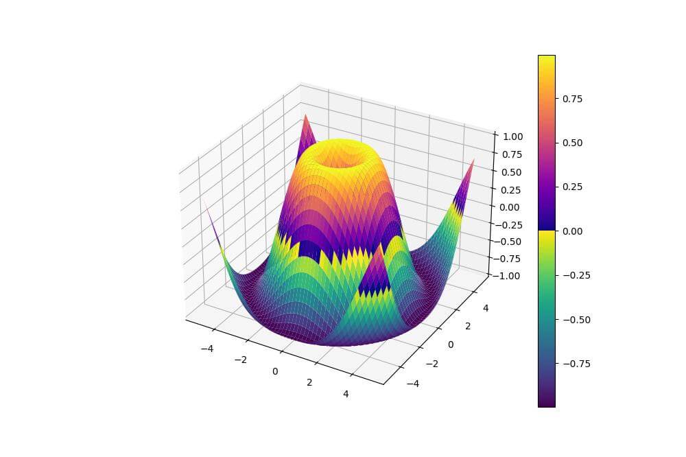
This code creates a custom colormap by blending the ‘viridis’ and ‘plasma’ colormaps.

The resulting plot uses this blended colormap to represent the Z-axis values.

 

Combine Multiple Colormaps in a Single Plot

You can use different colormaps for various elements in a single 3D plot to highlight different aspects of your data.

import numpy as np
import matplotlib.pyplot as plt
from mpl_toolkits.mplot3d import Axes3D
x = np.linspace(-5, 5, 100)
y = np.linspace(-5, 5, 100)
X, Y = np.meshgrid(x, y)
Z = np.sin(np.sqrt(X**2 + Y**2))
fig = plt.figure(figsize=(12, 8))
ax = fig.add_subplot(111, projection='3d')

# Plot surface with one colormap
surf = ax.plot_surface(X, Y, Z, cmap='viridis', alpha=0.7)

# Plot contours with another colormap
contours = ax.contourf(X, Y, Z, zdir='z', offset=-1, cmap='plasma', alpha=0.5)
fig.colorbar(surf, shrink=0.6, aspect=10, label='Surface')
fig.colorbar(contours, shrink=0.6, aspect=10, label='Contours')
plt.show()

Output:

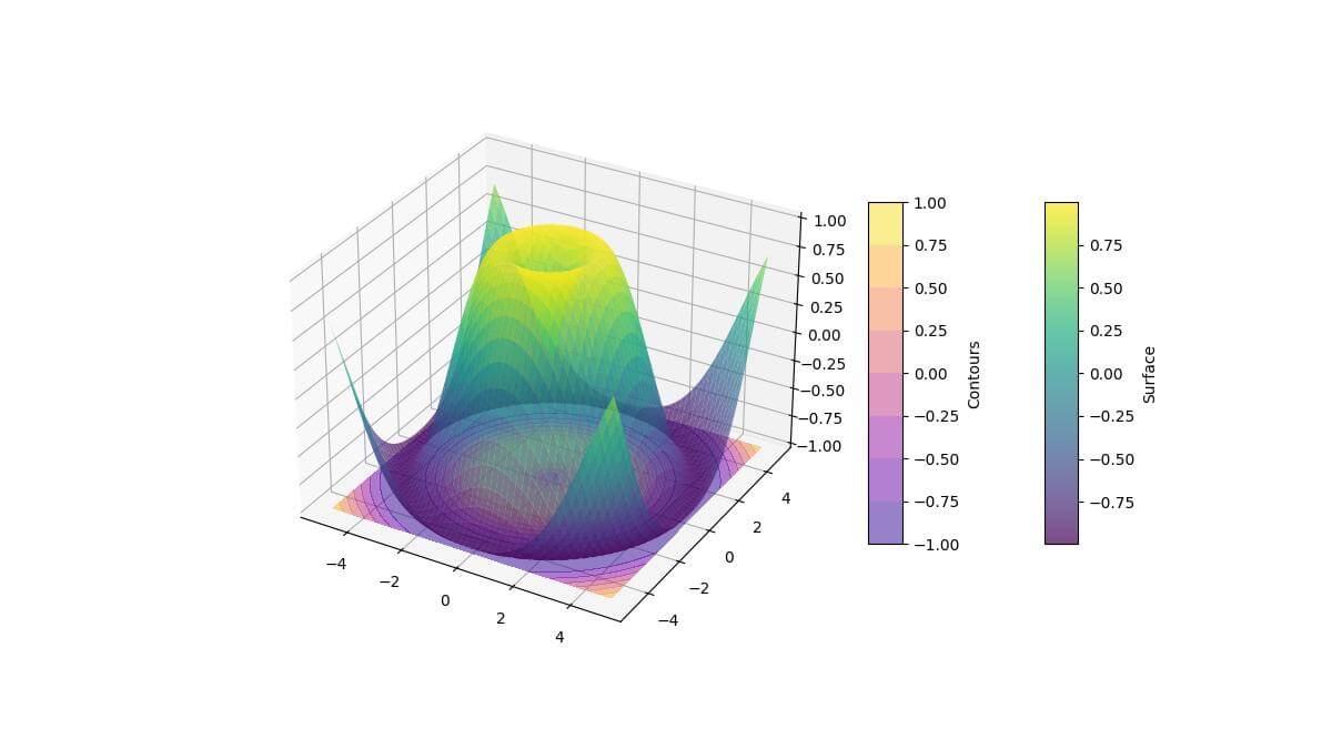
This code combines a surface plot using the ‘viridis’ colormap with contour plots using the ‘plasma’ colormap.

The contour plot is offset along the z-axis for better visibility.

 

Using ipywidgets for Dynamic Colormap Selection

You can create interactive 3D plots with dynamic colormap selection using ipywidgets in Jupyter notebooks.

import numpy as np
import matplotlib.pyplot as plt
from mpl_toolkits.mplot3d import Axes3D
import ipywidgets as widgets
from IPython.display import display
x = np.linspace(-5, 5, 100)
y = np.linspace(-5, 5, 100)
X, Y = np.meshgrid(x, y)
Z = np.sin(np.sqrt(X**2 + Y**2))
def update_plot(cmap):
  fig = plt.figure(figsize=(10, 8))
  ax = fig.add_subplot(111, projection='3d')
  surf = ax.plot_surface(X, Y, Z, cmap=cmap)
  fig.colorbar(surf)
  plt.show()

# Create a dropdown widget for colormap selection
cmap_dropdown = widgets.Dropdown(
  options=['viridis', 'plasma', 'inferno', 'magma', 'cividis'],
  value='viridis',
  description='Colormap:',
)

# Link the widget to the update function
interactive_plot = widgets.interactive(update_plot, cmap=cmap_dropdown)
display(interactive_plot)

Output:

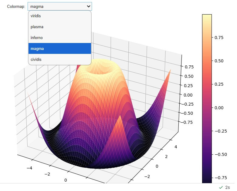
The plot updates in real-time as you select different colormaps.