Depth First Search algorithm in Python (Multiple Examples)

Depth First Search is a popular graph traversal algorithm. In this tutorial, We will understand how it works, along with examples; and how we can implement it in Python.
We will be looking at the following sections:

 

 

Introduction

Graphs and Trees are some of the most important data structures we use for various applications in Computer Science.
They represent data in the form of nodes, which are connected to other nodes through ‘edges’.

Like other data structures, traversing all the elements or searching for an element in a graph or a tree is one of the fundamental operations that is required to define such data structures. Depth First Search is one such graph traversal algorithm.

The Depth First Search Algorithm

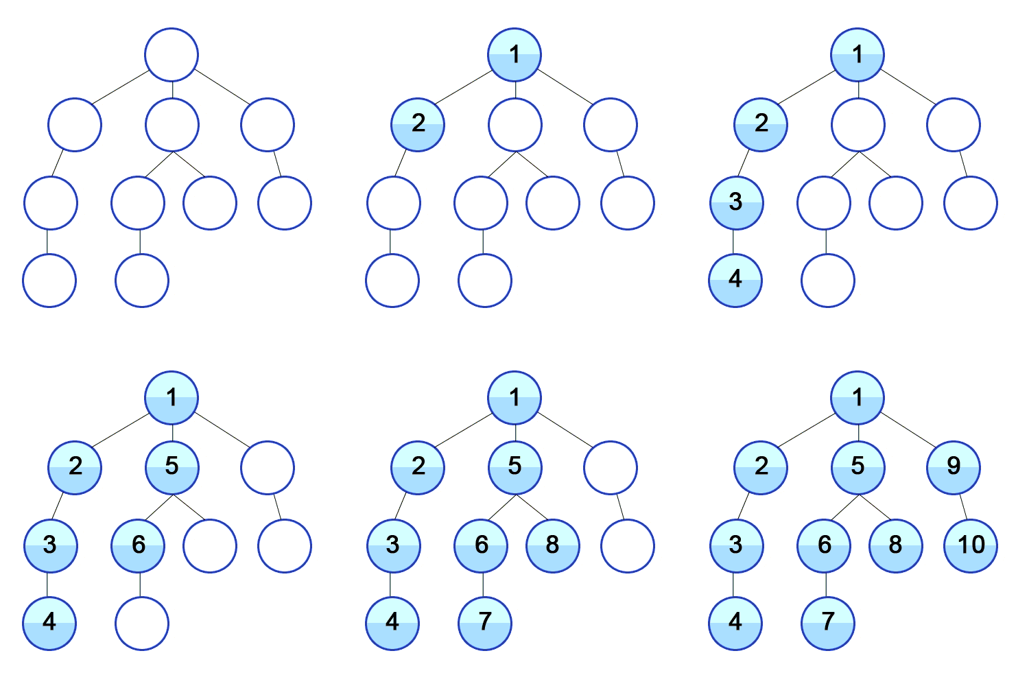
Depth First Search begins by looking at the root node (an arbitrary node) of a graph. If we are performing a traversal of the entire graph, it visits the first child of a root node, then, in turn, looks at the first child of this node and continues along this branch until it reaches a leaf node.

Next, it backtracks and explores the other children of the parent node in a similar manner. This continues until we visit all the nodes of the tree, and there is no parent node left to explore.

source: Wikipedia

However, if we are performing a search of a particular element, then at each step, a comparison operation will occur with the node we are currently at.
If the element is not present in a particular node, then the same process exploring each branch and backtracking takes place.

This continues until either all the nodes of the graph have been visited, or we have found the element we were looking for.

 

Representing a graph

Before we try to implement the DFS algorithm in Python, it is necessary to first understand how to represent a graph in Python.

There are various versions of a graph. A graph may have directed edges (defining the source and destination) between two nodes, or undirected edges. The edges between nodes may or may not have weights. Depending on the application, we may use any of the various versions of a graph.

For the purpose of traversal through the entire graph, we will use graphs with directed edges (since we need to model parent-child relation between nodes), and the edges will have no weights since all we care about is the complete traversal of the graph.

Now there are various ways to represent a graph in Python; two of the most common ways are the following:

1. Adjacency Matrix
2. Adjacency List

 

Adjacency Matrix

Adjacency Matrix is a square matrix of shape N x N (where N is the number of nodes in the graph).
Each row represents a node, and each of the columns represents a potential child of that node.
Each (row, column) pair represents a potential edge.

Whether or not the edge exists depends on the value of the corresponding position in the matrix.
A non-zero value at the position (i,j) indicates the existence of an edge between nodes i and j, while the value zero means there exists no edge between i and j.

The values in the adjacency matrix may either be a binary number or a real number.
We can use binary values in a non-weighted graph (1 means edge exists, and a 0 means it doesn’t).
For real values, we can use them for a weighted graph and represent the weight associated with the edge between the row and column representing the position.

E.g., a value 10 between at position (2,3) indicates there exists an edge bearing weight 10 between nodes 2 and 3.

In Python, we can represent the adjacency matrices using a 2-dimensional NumPy array.

 

Adjacency List

Adjacency List is a collection of several lists. Each list represents a node in the graph, and stores all the neighbors/children of this node.

In Python, an adjacency list can be represented using a dictionary where the keys are the nodes of the graph, and their values are a list storing the neighbors of these nodes.

We will use this representation for our implementation of the DFS algorithm.

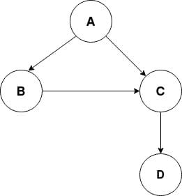
Let’s take an example graph and represent it using a dictionary in Python.

The given graph has the following four edges:

1. A -> B
2. A -> C
3. B -> C
4. C -> D

Let’s now create a dictionary in Python to represent this graph.

graph = {"A": ["B", "C"],
            "B": ["C"],
            "C": ["D"]}

Now that we know how to represent a graph in Python, we can move on to the implementation of the DFS algorithm.

Implementing Depth First Search(a non-recursive approach)

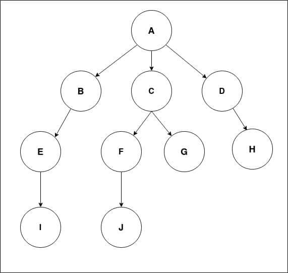
We will consider the graph example shown in the animation in the first section.

Let’s define this graph as an adjacency list using the Python dictionary.

graph = {"A":["D","C","B"],
   "B":["E"],
   "C":["G","F"],
   "D":["H"],
   "E":["I"],
   "F":["J"]}

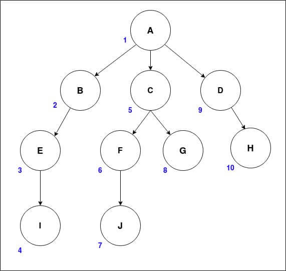
One of the expected orders of traversal for this graph using DFS would be:

Let’s implement a method that accepts a graph and traverses through it using DFS. We can achieve this using both recursion technique as well as non-recursive, iterative approach.
In this section, we’ll look at the iterative method.

We will use a stack and a list to keep track of the visited nodes.
We’ll begin at the root node, append it to the path and mark it as visited. Then we will add all of its neighbors to the stack.
At each step, we will pop out an element from the stack and check if it has been visited.
If it has not been visited, we’ll add it to the path and add all of its neighbors to the stack.

def dfs_non_recursive(graph, source):
       if source is None or source not in graph:
           return "Invalid input"
       path = []
       stack = [source]
       while(len(stack) != 0):
           s = stack.pop()
           if s not in path:
               path.append(s)
           if s not in graph:
               #leaf node
               continue
           for neighbor in graph[s]:
               stack.append(neighbor)
       return " ".join(path)

Our user-defined method takes the dictionary representing the graph and a source node as input.
Note that the source node has to be one of the nodes in the dictionary, else the method will return an “Invalid input” error.

Let’s call this method on our defined graph, and verify that the order of traversal matches with that demonstrated in the figure above.

DFS_path = dfs_non_recursive(graph, "A")
print(DFS_path)

Output :

Thus the order of traversal of the graph is in the ‘Depth First’ manner.

 

DFS using a recursive method

We can implement the Depth First Search algorithm using a popular problem-solving approach called recursion.

Recursion is a technique in which the same problem is divided into smaller instances, and the same method is recursively called within its body.

We will define a base case inside our method, which is – ‘If the leaf node has been visited, we need to backtrack’.

Let’s implement the method:

def recursive_dfs(graph, source,path = []):
       if source not in path:
           path.append(source)
           if source not in graph:
               # leaf node, backtrack
               return path
           for neighbour in graph[source]:
               path = recursive_dfs(graph, neighbour, path)
       return path

Now we can create our graph (same as in the previous section), and call the recursive method.

graph = {"A":["B","C", "D"],
           "B":["E"],
           "C":["F","G"],
           "D":["H"],
           "E":["I"],
           "F":["J"]}
path = recursive_dfs(graph, "A")
print(" ".join(path))

Output:

The order of traversal is again in the Depth-First manner.

 

Depth First Search on a Binary Tree

What is a Binary Tree?

A binary tree is a special kind of graph in which each node can have only two children or no child.
Another important property of a binary tree is that the value of the left child of the node will be less than or equal to the current node’s value.
Similarly, the value in the right child is greater than the current node’s value.

Thus every value in the left branch of the root node is smaller than the value at the root, and those in the right branch will have a value greater than that at the root.

Let’s understand how we can represent a binary tree using Python classes.

 

Representing Binary Trees using Python classes

We can create a class to represent each node in a tree, along with its left and right children.
Using the root node object, we can parse the whole tree.

We will also define a method to insert new values into a binary tree.

class Node:
       def __init__(self, value):
           self.value = value
           self.left = None
           self.right = None
       def insert(self, value):
           if value:
               if value < self.value:
                   if self.left is None:
                       self.left = Node(value)
                   else:
                       self.left.insert(value)
               elif value > self.value:
                   if self.right is None:
                       self.right = Node(value)
                   else:
                       self.right.insert(value)
               else:
                   self.value = value

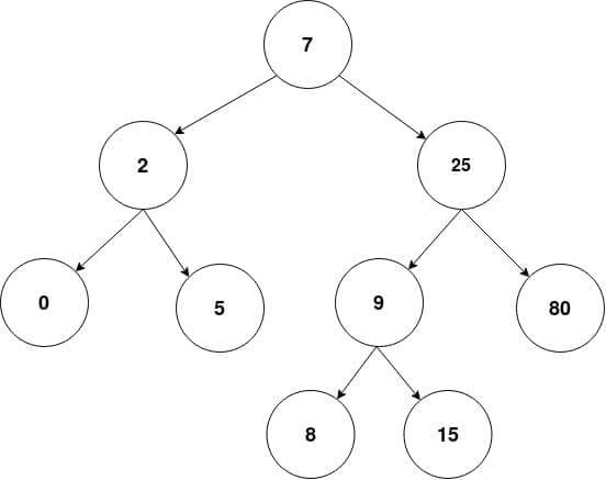
Let’s now create a root node object and insert values in it to construct a binary tree like the one shown in the figure in the previous section.

root = Node(7)
root.insert(2)
root.insert(25)
root.insert(9)
root.insert(80)
root.insert(0)
root.insert(5)
root.insert(15)
root.insert(8)

This will construct the binary tree shown in the figure above.
It will also ensure that the properties of binary trees i.e, ‘2 children per node’ and ‘left < root < right’ are satisfied no matter in what order we insert the values.

 

Implementing DFS for a binary tree

Let’s now define a recursive function that takes as input the root node and displays all the values in the tree in the ‘Depth First Search’ order.

def dfs_binary_tree(root):
       if root is None:
           return
       else:
           print(root.value,end=" ")
           dfs_binary_tree(root.left)
           dfs_binary_tree(root.right)

We can now call this method and pass the root node object we just created.

dfs_binary_tree(root)

Output:

This order is also called as the ‘preorder traversal’ of a binary tree.

 

Depth First Search using networkx

So far, we have been writing our logic for representing graphs and traversing them.
But, like all other important applications, Python offers a library to handle graphs as well. It is called ‘networkx’.

‘networkx’ is a Python package to represent graphs using nodes and edges, and it offers a variety of methods to perform different operations on graphs, including the DFS traversal.

Let’s first look at how to construct a graph using networkx.

 

Constructing a graph in networkx

To construct a graph in networkx, we first create a graph object and then add all the nodes in the graph using the ‘add_node()’ method, followed by defining all the edges between the nodes, using the ‘add_edge()’ method.

Let’s construct the following graph using ‘networkx’.

import networkx as nx
G = nx.Graph() #create a graph
G.add_node(1) # add single node
G.add_node(2)
G.add_node(3)
G.add_node(4)
G.add_node(5)
G.add_nodes_from([6,7,8,9]) #add multiple nodes

Now that we have added all the nodes let’s define the edges between these nodes as shown in the figure.

# adding edges
G.add_edge(5,8)
G.add_edge(5,4)
G.add_edge(5,7)
G.add_edge(8,2)
G.add_edge(4,3)
G.add_edge(4,1)
G.add_edge(7,6)
G.add_edge(6,9)

 

Visualizing the graph in DFS

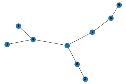
Now, we constructed the graph by defining the nodes and edges let’s see how it looks the networkx’s ‘draw()’ method and verify if it is constructed the way we wanted it to be. We will use matplotlib to show the graph.

import matplotlib.pyplot as plt
nx.draw(G, with_labels=True, font_weight='bold')
plt.show()

Output:

The orientation may be a little different than our design, but it resembles the same graph, with the nodes and the same edges between them.

Let’s now perform DFS traversal on this graph.

 

Graph traversal in networkx – DFS

The ‘networkx’ offers a range of methods for traversal of the graph in different ways. We will use the ‘dfs_preorder_nodes()’ method to parse the graph in the Depth First Search order.

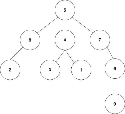
The expected order from the figure should be:
5, 8, 2, 4, 3, 1, 7, 6, 9

Let’s call the method and see in what order it prints the nodes.

dfs_output = list(nx.dfs_preorder_nodes(G, source=5))
print(dfs_output)

Output:

Thus the order of traversal by networkx is along our expected lines.

Now that we have understood the depth-first search or DFS traversal well, let’s look at some of its applications.

 

Topological sorting using Depth First Search

Topological sorting is one of the important applications of graphs used to model many real-life problems where the beginning of a task is dependent on the completion of some other task.

For instance, we may represent a number of jobs or tasks using nodes of a graph.
Some of the tasks may be dependent on the completion of some other task. This dependency is modeled through directed edges between nodes.
A graph with directed edges is called a directed graph.

If we want to perform a scheduling operation from such a set of tasks, we have to ensure that the dependency relation is not violated i.e, any task that comes later in a chain of tasks is always performed only after all the tasks before it has finished.
We can achieve this kind of order through the topological sorting of the graph.

Note that for topological sorting to be possible, there has to be no directed cycle present in the graph, that is, the graph has to be a directed acyclic graph or DAG.

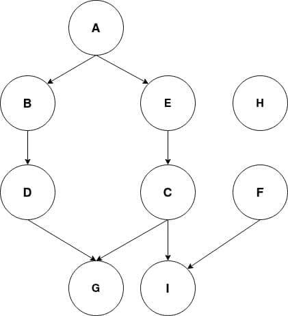
Let’s take an example of a DAG and perform topological sorting on it, using the Depth First Search approach.

Let’s say each node in the above graph represents a task in a factory to produce a product. The directed arrows between the nodes model are the dependencies of each task on the completion of the previous tasks.

Hence whatever ordering of tasks we chose to perform, to begin the task C, tasks A and E must have been completed.

Similarly, for performing the task I, the tasks A, E, C, and F must have been completed. Since there is no inward arrow on node H, the task H can be performed at any point without the dependency on completion of any other task.

We can construct such a directed graph using Python networkx’s ‘digraph’ module.

dag = nx.digraph.DiGraph()
dag.add_nodes_from(['A', 'B', 'C', 'D', 'E', 'F', 'G', 'H', 'I'])
dag.add_edges_from([('A', 'B'), ('A', 'E'), ('B', 'D'), ('E', 'C'),
                      ('D', 'G'),('C', 'G'),('C', 'I'), ('F', 'I')])

Note that we have used the methods ‘add_nodes_from()’ and ‘add_edges_from()’ to add all the nodes and edges of the directed graph at once.

We can now write a function to perform topological sorting using DFS.

We will begin at a node with no inward arrow, and keep exploring one of its branches until we hit a leaf node, and then we backtrack and explore other branches.

Once we explore all the branches of a node, we will mark the node as ‘visited’ and push it to a stack.

Once every node is visited, we can perform repeated pop operations on the stack to give us a topologically sorted ordering of the tasks.

Now let’s translate this idea into a Python function:

def dfs(dag, start, visited, stack):
       if start in visited:
           # node and all its branches have been visited
           return stack, visited
       if dag.out_degree(start) == 0:
           # if leaf node, push and backtrack
           stack.append(start)
           visited.append(start)
           return stack, visited
       #traverse all the branches
       for node in dag.neighbors(start):
           if node in visited:
               continue
           stack, visited = dfs(dag, node, visited, stack)
       #now, push the node if not already visited
       if start not in visited:
           print("pushing %s"%start)
           stack.append(start)
           visited.append(start)
       return stack, visited
   def topological_sort_using_dfs(dag):
       visited = []
       stack=[]
       start_nodes = [i for i in dag.nodes if dag.in_degree(i)==0]
   #     print(start_nodes)
       for s in start_nodes:
           stack, visited = dfs(dag, s, visited, stack)
       print("Topological sorted:")
       while(len(stack)!=0):
           print(stack.pop(), end=" ")

We have defined two functions – one for recursive traversal of a node, and the main topological sort function that first finds all nodes with no dependency and then traverses each of them using the Depth First Search approach.
Finally, it pops out values from the stack, which produces a topological sorting of the nodes.

Let’s now call the function ‘topological_sort_using_dfs()’

topological_sort_using_dfs(dag)

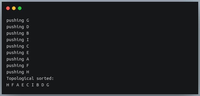
Output :

If we look closely at the output order, we’ll find that whenever each of the jobs starts, it has all its dependencies completed before it.

We can also compare this with the output of a topological sort method included in the ‘networkx’ module called ‘topological_sort()’.

topological_sorting = nx.topological_sort(dag)
for n in topological_sorting:
    print(n, end=' ')

Output:

It looks like the ordering produced by the networkx’s sort method is the same as the one produced by our method.

 

Finding connected components using DFS

A graph has another important property called the connected components. A connected component in an undirected graph refers to a set of nodes in which each vertex is connected to every other vertex through a path.

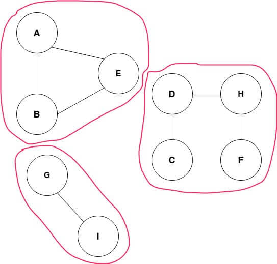
Let’s look at the following example:

In the graph shown above, there are three connected components; each of them has been marked in pink.

Let’s construct this graph in Python, and then chart out a way to find connected components in it.

graph = nx.Graph()
graph.add_nodes_from(['A', 'B', 'C', 'D', 'E', 'F', 'G', 'H', 'I'])
graph.add_edges_from([('A', 'B'), ('B', 'E'), ('A', 'E')]) #component 1
graph.add_edges_from([('C', 'D'), ('D', 'H'), ('H', 'F'), ('F', 'C')]) #component 2
graph.add_edge('G','I') #component 3

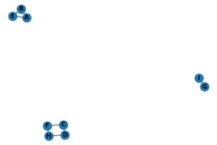
Let’s also visualize it while we are at it.

import matplotlib.pyplot as plt
nx.draw(graph, with_labels=True, font_weight='bold')
plt.show()

Output:

To find connected components using DFS, we will maintain a common global array called ‘visited’, and every time we encounter a new variable that has not been visited, we will start finding which connected component it is a part of.

We will mark every node in that component as ‘visited’ so we will not be able to revisit it to find another connected component.

We will repeat this procedure for every node, and the number of times we called the DFS method to find connected components from a node, will be equal to the number of connected components in the graph.

Let’s write this logic in Python and run it on the graph we just constructed:

def find_connected_components(graph):
       visited = []
       connected_components = []
       for node in graph.nodes:
           if node not in visited:
               cc = [] #connected component
               visited, cc = dfs_traversal(graph, node, visited, cc)
               connected_components.append(cc)
       return connected_components
   def dfs_traversal(graph, start, visited, path):
       if start in visited:
           return visited, path
       visited.append(start)
       path.append(start)
       for node in graph.neighbors(start):
           visited, path = dfs_traversal(graph, node, visited, path)
       return visited, path

Let’s use our method on the graph we constructed in the previous step.

connected_components = find_connected_components(graph)
print("Total number of connected components =", len(connected_components))
for cc in connected_components:
    print(cc)

Output:

 

Conclusion

In this blog, we understood the DFS algorithm and used it in different ways.

We began by understanding how a graph can be represented using common data structures and implemented each of them in Python.

We then implemented the Depth First Search traversal algorithm using both the recursive and non-recursive approach.

Next, we looked at a special form of a graph called the binary tree and implemented the DFS algorithm on the same.
Here we represented the entire tree using node objects constructed from the Python class we defined to represent a node.

Then we looked at Python’s offering for representing graphs and performing operations on them – the ‘networkx’ module.
We used it to construct a graph, visualize it, and run our DFS method on it. We compared the output with the module’s own DFS traversal method.

Finally, we looked at two important applications of the Depth First Search traversal namely, topological sort and finding connected components in a graph.