Create 3D Spline Plots in Python using Matplotlib

Splines allow you to create smooth curves and surfaces in 3D space.

In this tutorial, you’ll learn how to create various types of 3D spline plots using Python.

You’ll explore different spline types, from basic curves to more complex surfaces, using Python libraries like NumPy, SciPy, and Matplotlib.

 

 

Basic 3D Spline Curve

To create a basic 3D spline curve, you can use the SciPy interpolate module.

Here’s how to generate and plot a simple 3D spline curve:

import numpy as np
from scipy import interpolate
import matplotlib.pyplot as plt
x = np.array([0, 1, 2, 3, 4, 5])
y = np.array([0, 2, 1, 3, 2, 4])
z = np.array([0, 1, 2, 0, 1, 0])

# Create a 3D spline
tck, u = interpolate.splprep([x, y, z], s=0)

# Generate points on the spline
u_new = np.linspace(0, 1, 100)
x_new, y_new, z_new = interpolate.splev(u_new, tck)
fig = plt.figure()
ax = fig.add_subplot(111, projection='3d')
ax.plot(x_new, y_new, z_new, label='Spline')
ax.scatter(x, y, z, c='red', label='Control points')
ax.set_xlabel('X')
ax.set_ylabel('Y')
ax.set_zlabel('Z')
ax.legend()
plt.show()

Output:

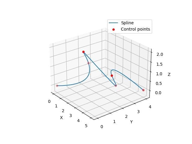
This code creates a 3D spline curve using control points.

The splprep function generates a spline representation, which is then evaluated using splev to create smooth curve points.

 

3D B-spline Surface

You can create a 3D B-spline surface using SciPy RectBivariateSpline:

import numpy as np
from scipy.interpolate import RectBivariateSpline
import matplotlib.pyplot as plt

# Generate sample data
x = np.linspace(0, 10, 10)
y = np.linspace(0, 10, 10)
X, Y = np.meshgrid(x, y)
Z = np.sin(X) * np.cos(Y)
spline = RectBivariateSpline(x, y, Z)

# Generate a finer grid for smooth plotting
x_fine = np.linspace(0, 10, 100)
y_fine = np.linspace(0, 10, 100)
X_fine, Y_fine = np.meshgrid(x_fine, y_fine)
Z_fine = spline(x_fine, y_fine)
fig = plt.figure(figsize=(10, 8))
ax = fig.add_subplot(111, projection='3d')
surf = ax.plot_surface(X_fine, Y_fine, Z_fine, cmap='viridis')
ax.set_xlabel('X')
ax.set_ylabel('Y')
ax.set_zlabel('Z')
fig.colorbar(surf)
plt.show()

Output:

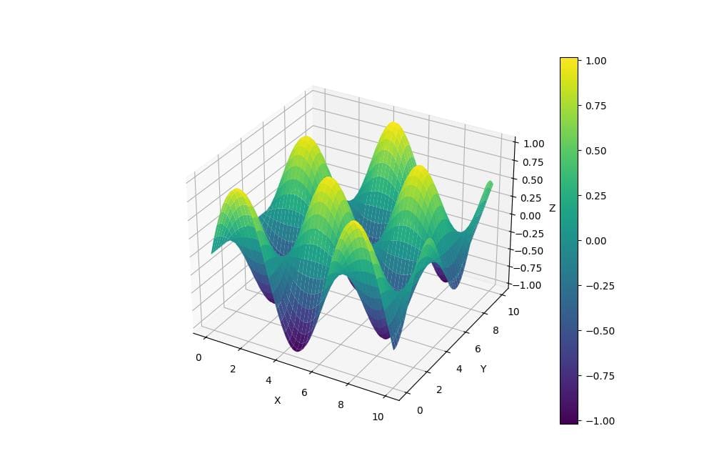
This code creates a 3D B-spline surface using a sine-cosine function as sample data.

The RectBivariateSpline function generates a smooth surface interpolation, which is then plotted on a finer grid for better visualization.

 

Parametric 3D Spline

You can create a parametric 3D spline using NumPy and Matplotlib:

import numpy as np
import matplotlib.pyplot as plt
from mpl_toolkits.mplot3d import Axes3D

# Define parametric equations
def x(t):
    return np.cos(t)
def y(t):
    return np.sin(t)
def z(t):
    return t
t = np.linspace(0, 4*np.pi, 100)
x_vals = x(t)
y_vals = y(t)
z_vals = z(t)
fig = plt.figure()
ax = fig.add_subplot(111, projection='3d')
ax.plot(x_vals, y_vals, z_vals)
ax.set_xlabel('X')
ax.set_ylabel('Y')
ax.set_zlabel('Z')
plt.show()

Output:

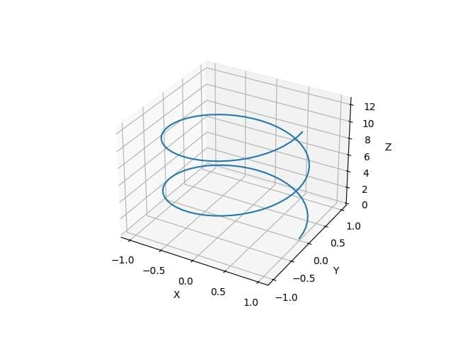
This code creates a parametric 3D spline by defining separate functions for x, y, and z coordinates.

 

Closed 3D Spline Loop

To create a closed 3D spline loop, you can use SciPy splprep and splev functions with periodic boundary conditions:

import numpy as np
from scipy import interpolate
import matplotlib.pyplot as plt

# Define control points for a closed loop
theta = np.linspace(0, 2*np.pi, 8, endpoint=False)
x = np.cos(theta) + 0.1 * np.random.randn(8)
y = np.sin(theta) + 0.1 * np.random.randn(8)
z = np.sin(2*theta) + 0.1 * np.random.randn(8)

# Create a periodic spline
tck, u = interpolate.splprep([x, y, z], s=0, per=True)

# Generate points on the spline
u_new = np.linspace(0, 1, 100)
x_new, y_new, z_new = interpolate.splev(u_new, tck)
fig = plt.figure()
ax = fig.add_subplot(111, projection='3d')
ax.plot(x_new, y_new, z_new, label='Closed spline')
ax.scatter(x, y, z, c='red', label='Control points')
ax.set_xlabel('X')
ax.set_ylabel('Y')
ax.set_zlabel('Z')
ax.legend()
plt.show()

Output:

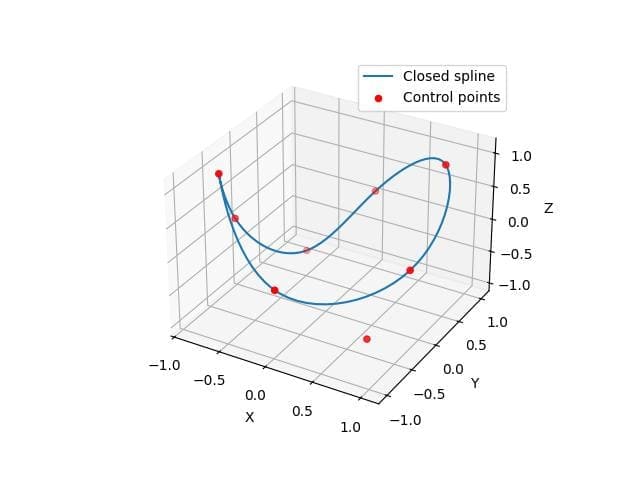
This code creates a closed 3D spline loop by setting the per=True parameter in splprep.

 

3D Catmull-Rom Spline

To create a 3D Catmull-Rom spline, you can implement the algorithm manually using NumPy:

import numpy as np
import matplotlib.pyplot as plt
def catmull_rom_spline(P0, P1, P2, P3, num_points=100):
    """Compute Catmull-Rom spline between P1 and P2."""
    alpha = 0.5
    t = np.linspace(0, 1, num_points)
    t = t.reshape(num_points, 1)
    A = np.array([
        [0, 1, 0, 0],
        [-alpha, 0, alpha, 0],
        [2*alpha, alpha-3, 3-2*alpha, -alpha],
        [-alpha, 2-alpha, alpha-2, alpha]
    ])
    points = np.array([P0, P1, P2, P3])
    return (t**np.arange(4)).dot(A).dot(points)

# Define control points
control_points = np.array([
    [0, 0, 0],
    [1, 1, 1],
    [2, -1, 2],
    [3, 0, -1],
    [4, 1, 0]
])

# Generate spline segments
spline_points = []
for i in range(len(control_points) - 3):
    spline_points.append(catmull_rom_spline(
        control_points[i],
        control_points[i+1],
        control_points[i+2],
        control_points[i+3]
    ))

# Combine spline segments
spline = np.vstack(spline_points)
fig = plt.figure()
ax = fig.add_subplot(111, projection='3d')
ax.plot(spline[:, 0], spline[:, 1], spline[:, 2], label='Catmull-Rom spline')
ax.scatter(control_points[:, 0], control_points[:, 1], control_points[:, 2], c='red', label='Control points')
ax.set_xlabel('X')
ax.set_ylabel('Y')
ax.set_zlabel('Z')
ax.legend()
plt.show()

Output:

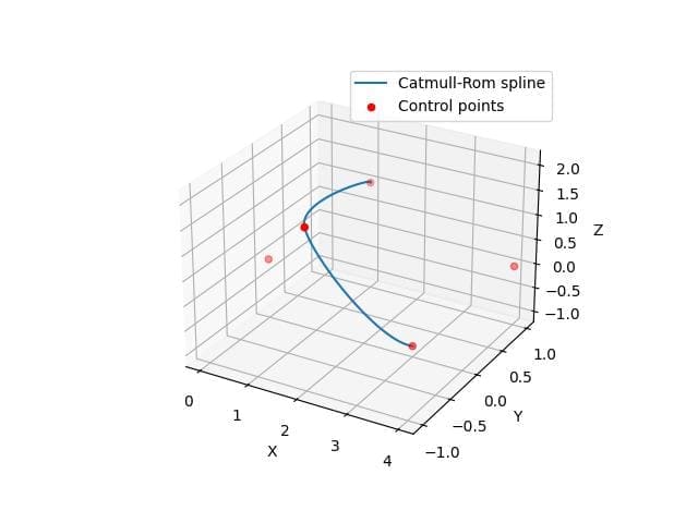
This code generates smooth curve segments between control points.

 

Hermite spline in 3D space

To create a Hermite spline in 3D space, you can implement the algorithm manually:

import numpy as np
import matplotlib.pyplot as plt
def hermite_spline(P0, P1, T0, T1, num_points=100):
    """Compute Hermite spline between P0 and P1 with tangents T0 and T1."""
    t = np.linspace(0, 1, num_points).reshape(-1, 1)

    H00 = 2*t**3 - 3*t**2 + 1
    H10 = t**3 - 2*t**2 + t
    H01 = -2*t**3 + 3*t**2
    H11 = t**3 - t**2
    return H00 * P0 + H10 * T0 + H01 * P1 + H11 * T1

# Define control points and tangents
P0 = np.array([0, 0, 0])
P1 = np.array([3, 4, 2])
T0 = np.array([1, 2, 1])
T1 = np.array([2, -1, 1])
spline = hermite_spline(P0, P1, T0, T1)
fig = plt.figure()
ax = fig.add_subplot(111, projection='3d')
ax.plot(spline[:, 0], spline[:, 1], spline[:, 2], label='Hermite spline')
ax.scatter([P0[0], P1[0]], [P0[1], P1[1]], [P0[2], P1[2]], c='red', label='Control points')
ax.quiver(P0[0], P0[1], P0[2], T0[0], T0[1], T0[2], color='green', label='Tangents')
ax.quiver(P1[0], P1[1], P1[2], T1[0], T1[1], T1[2], color='green')
ax.set_xlabel('X')
ax.set_ylabel('Y')
ax.set_zlabel('Z')
ax.legend()
plt.show()

Output:

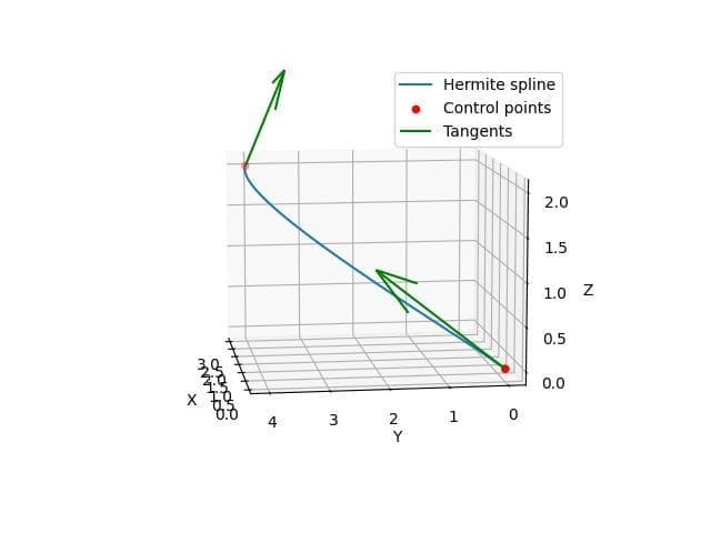
This code plots a 3D Hermite spline between two points with specified tangent vectors.

The resulting curve smoothly interpolates between the points while respecting the given tangents.