How to Create 3D Wireframe Plot in Python

In this tutorial, you’ll learn how to create 3D wireframe plots in Python using various libraries and methods.

Wireframe plots are excellent for visualizing 3D surfaces and understanding the structure of complex data.

You’ll explore different methods, from matplotlib to more advanced libraries like Plotly, Mayavi, PyVista, and VisPy.

 

 

Using plot_wireframe()

To create a basic 3D wireframe plot, you can use the matplotlib plot_wireframe() function. Here’s how to do it:

import numpy as np
import matplotlib.pyplot as plt

# Sample data
x = np.linspace(-5, 5, 50)
y = np.linspace(-5, 5, 50)
X, Y = np.meshgrid(x, y)
Z = np.sin(np.sqrt(X**2 + Y**2))
fig = plt.figure(figsize=(10, 8))
ax = fig.add_subplot(111, projection='3d')
ax.plot_wireframe(X, Y, Z, color='blue')
ax.set_xlabel('X')
ax.set_ylabel('Y')
ax.set_zlabel('Z')
ax.set_title('3D Wireframe Plot using matplotlib')
plt.show()

Output:

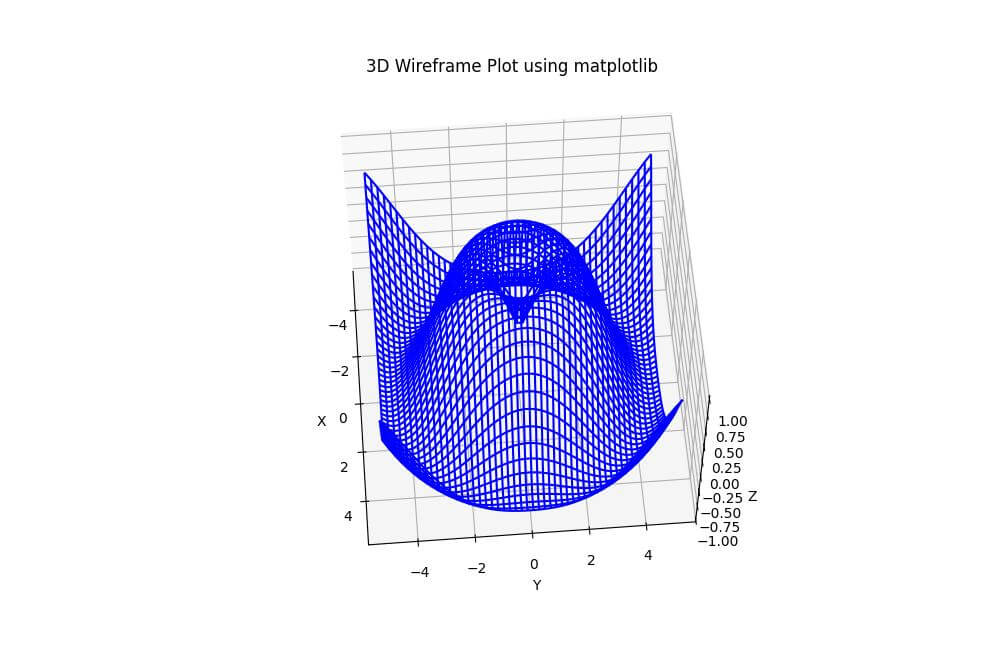
The plot_wireframe() function takes the X, Y, and Z coordinates as input and creates a wireframe representation of the surface.

The resulting plot shows the structure of the sinusoidal function in 3D space.

 

Using plot_surface()

You can also create a wireframe-style plot using the matplotlib plot_surface() function with custom parameters:

import numpy as np
import matplotlib.pyplot as plt
x = np.linspace(-5, 5, 50)
y = np.linspace(-5, 5, 50)
X, Y = np.meshgrid(x, y)
Z = np.cos(X) * np.sin(Y)
fig = plt.figure(figsize=(10, 8))
ax = fig.add_subplot(111, projection='3d')
ax.plot_surface(X, Y, Z, rstride=1, cstride=1, color='cyan', edgecolor='black', linewidth=0.3)
ax.set_xlabel('X')
ax.set_ylabel('Y')
ax.set_zlabel('Z')
ax.set_title('3D Wireframe-style Plot using plot_surface()')
plt.show()

Output:

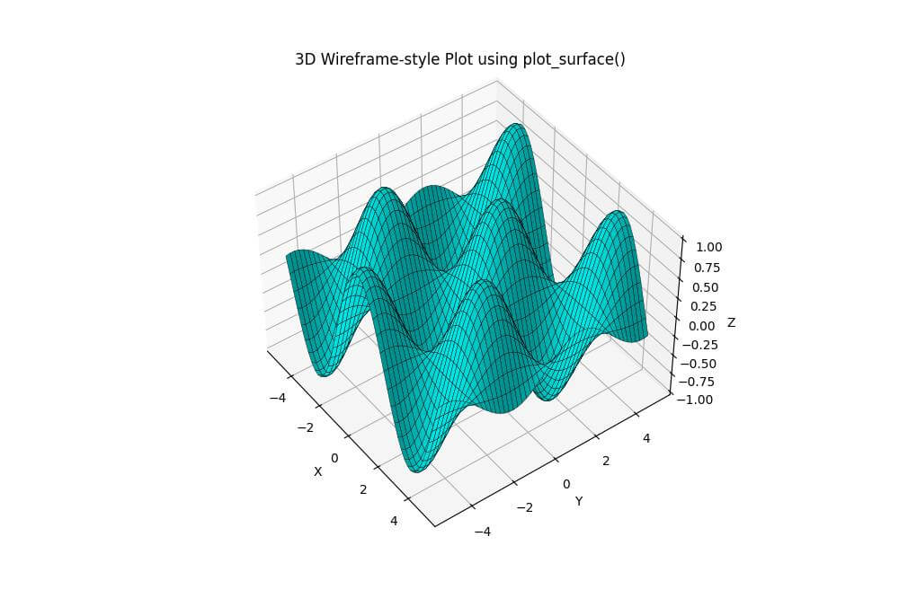
The plot_surface() function is used with custom parameters rstride and cstride to control the density of the wireframe.

The edgecolor and linewidth parameters are set to create visible lines on the surface to give a wireframe-like look.

The resulting plot shows a cosine-sine surface with a cyan color and black wireframe lines.

 

Using plotly go.Surface()

For interactive 3D wireframe plots, you can use Plotly go.Surface() function:

import numpy as np
import plotly.graph_objects as go
x = np.linspace(-5, 5, 20)
y = np.linspace(-5, 5, 20)
X, Y = np.meshgrid(x, y)
Z = np.sin(X) * np.cos(Y)
fig = go.Figure(data=[go.Surface(x=X, y=Y, z=Z, 
                                 colorscale=[[0, 'rgb(0,0,255)'], [1, 'rgb(0,0,255)']],
                                 showscale=False)])
fig.update_traces(contours_x=dict(show=True, highlight=False, color="black"),
                  contours_y=dict(show=True, highlight=False, color="black"),
                  contours_z=dict(show=True, highlight=False, color="black"),
                  surfacecolor=None)
fig.update_layout(scene=dict(xaxis_title='X', yaxis_title='Y', zaxis_title='Z'),
                  title='3D Wireframe Plot using Plotly',
                  scene_camera=dict(eye=dict(x=1.5, y=-1.5, z=0.8)))
fig.show()

Output:

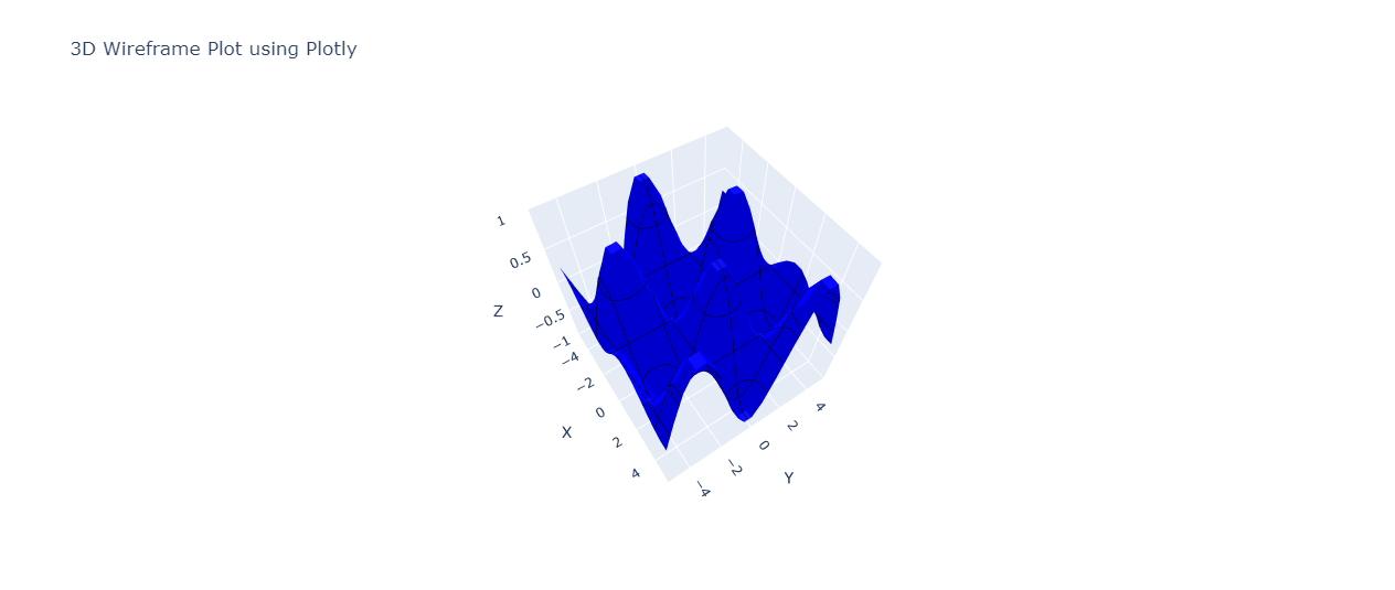
The update_traces adds black contour lines in all three dimensions (x, y, z) and removes the surface color to create a wireframe effect.
The plot shows a sinusoidal surface with a blue color and black wireframe lines.

 

Using Mayavi mlab.mesh()

You can use Mayavi mlab.mesh() function with a wireframe representation:

import numpy as np
from mayavi import mlab
x = np.linspace(-5, 5, 50)
y = np.linspace(-5, 5, 50)
X, Y = np.meshgrid(x, y)
Z = np.exp(-(X**2 + Y**2) / 10)
mlab.figure(size=(800, 600))
mlab.mesh(X, Y, Z, representation='wireframe', color=(0, 1, 0))
mlab.xlabel('X')
mlab.ylabel('Y')
mlab.zlabel('Z')
mlab.title('3D Wireframe Plot using Mayavi')
mlab.show()

Output:

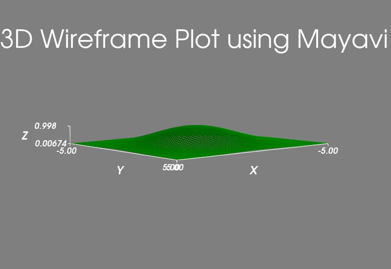
The mlab.mesh() function is used with representation=’wireframe’ to create a wireframe representation of the surface.

The resulting plot shows a Gaussian surface with green wireframe lines.

 

Using PyVista plot_wireframe()

PyVista offers a simple way to create 3D wireframe plots with its plot_wireframe() method:

import numpy as np
import pyvista as pv
x = np.linspace(-5, 5, 50)
y = np.linspace(-5, 5, 50)
X, Y = np.meshgrid(x, y)
Z = np.sin(X) * np.cos(Y)
grid = pv.StructuredGrid(X, Y, Z)
plotter = pv.Plotter()
plotter.add_mesh(grid, style='wireframe', color='red', line_width=2)
plotter.show_axes()
plotter.add_title('3D Wireframe Plot using PyVista')
plotter.show()

Output:

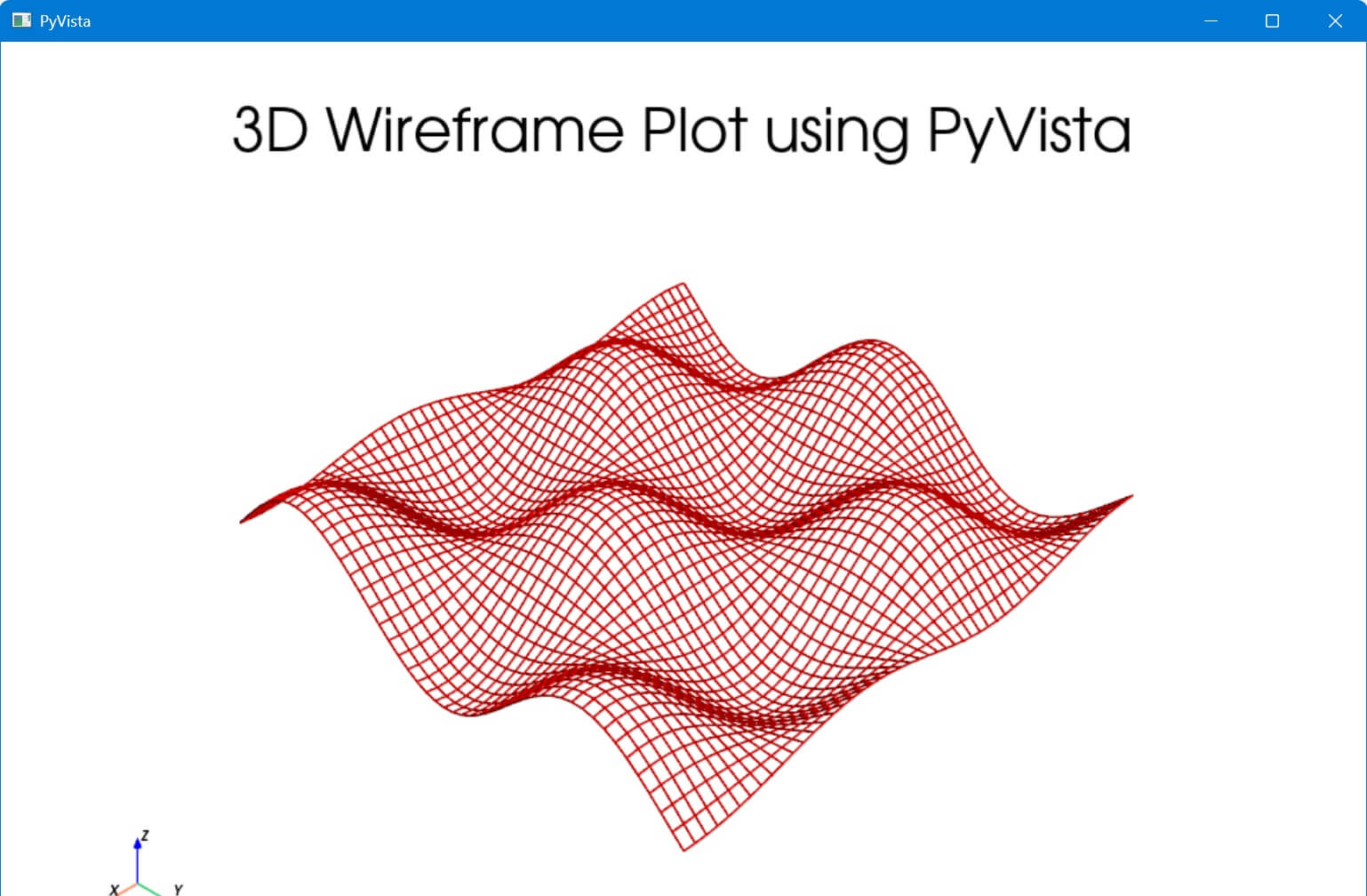
The pv.StructuredGrid() function is used to create a grid from the X, Y, and Z data, and the plot_wireframe() method is applied to render the wireframe.

The resulting plot shows a sinusoidal surface with red wireframe lines.

 

Using VisPy WireframeVisual class

For low-level control over 3D wireframe rendering, you can use VisPy WireframeVisual class:

import numpy as np
from vispy import app, scene
canvas = scene.SceneCanvas(keys='interactive', show=True)
view = canvas.central_widget.add_view()
view.camera = 'turntable'
x = np.linspace(-5, 5, 50)
y = np.linspace(-5, 5, 50)
x, y = np.meshgrid(x, y)
z = np.sin(np.sqrt(x**2 + y**2))
vertices = np.c_[x.ravel(), y.ravel(), z.ravel()]
rows, cols = x.shape
faces = []
for i in range(rows - 1):
    for j in range(cols - 1):
        # Create two triangles for each grid square
        faces.append([i * cols + j, i * cols + j + 1, (i + 1) * cols + j])
        faces.append([(i + 1) * cols + j, i * cols + j + 1, (i + 1) * cols + j + 1])
faces = np.array(faces)

# Create a mesh visual with wireframe mode
mesh = scene.visuals.Mesh(vertices=vertices,
                          faces=faces,
                          color='white',
                          mode='lines')  # 'lines' mode for wireframe
view.add(mesh)

# Add a grid for better visualization
grid = scene.visuals.GridLines(color='gray')
view.add(grid)
if __name__ == '__main__':
    app.run()

Output:

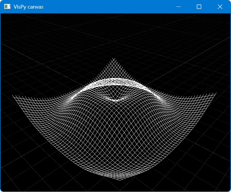
We create a grid of points using NumPy meshgrid and calculate the z-values using a sine function.

The vertices are the points on the grid, and the faces are created by connecting these points to form triangles.

Each square in the grid is divided into two triangles.

The Mesh visual is used to render the surface. By setting the mode to 'lines', the mesh is displayed as a wireframe.