Create 3D Polar Plots in Python using Matplotlib

In this tutorial, you’ll learn how to create 3D polar plots using Python.

You’ll use the matplotlib library to visualize data in a three-dimensional polar coordinate system.

This method is useful for representing cyclical or radial data in fields like physics, engineering, and data science.

 

 

Generate Data for 3D Polar Plot

To begin, you’ll need to generate data for your 3D polar plot.

Use NumPy to create arrays for radius, theta, and phi:

import numpy as np
import matplotlib.pyplot as plt
r = np.linspace(0, 5, 50)
theta = np.linspace(0, 2 * np.pi, 100)
r, theta = np.meshgrid(r, theta)
phi = np.linspace(0, np.pi, 50)

This code sets up the basic coordinate arrays for your 3D polar plot.

 

3D Polar Scatter Plot

To create a 3D polar scatter plot, you can use the scatter function:

fig = plt.figure(figsize=(10, 8))
ax = fig.add_subplot(111, projection='3d')
r = np.random.rand(100) * 5
theta = np.random.rand(100) * 2 * np.pi
z = np.random.rand(100) * 5
ax.scatter(r * np.cos(theta), r * np.sin(theta), z, c=z, cmap='plasma')
ax.set_xlabel('X')
ax.set_ylabel('Y')
ax.set_zlabel('Z')
plt.show()

Output:

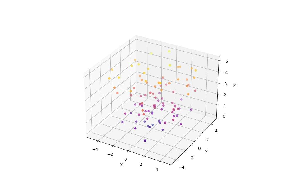
This code generates a 3D scatter plot with random data points in polar coordinates.

 

3D Polar Line Plot

For a 3D polar line plot, you can use the plot function:

fig = plt.figure(figsize=(10, 8))
ax = fig.add_subplot(111, projection='3d')
theta = np.linspace(0, 10 * np.pi, 1000)
r = theta ** 0.5
z = np.linspace(0, 5, 1000)
ax.plot(r * np.cos(theta), r * np.sin(theta), z, label='Spiral')
ax.legend()
ax.set_xlabel('X')
ax.set_ylabel('Y')
ax.set_zlabel('Z')
plt.show()

Output:

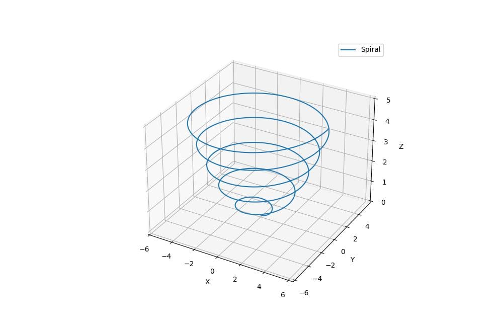
This code creates a 3D spiral line plot in polar coordinates.

 

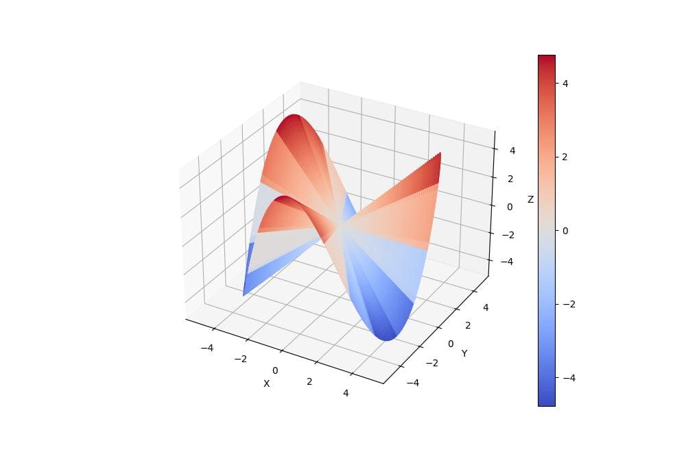
3D Polar Surface Plot

To create a 3D polar surface plot, you can use the plot_surface function:

fig = plt.figure(figsize=(10, 8))
ax = fig.add_subplot(111, projection='3d')
r = np.linspace(0, 5, 50)
theta = np.linspace(0, 2 * np.pi, 100)
r, theta = np.meshgrid(r, theta)
z = r * np.sin(3 * theta)
surf = ax.plot_surface(r * np.cos(theta), r * np.sin(theta), z, cmap='coolwarm')
fig.colorbar(surf)
ax.set_xlabel('X')
ax.set_ylabel('Y')
ax.set_zlabel('Z')
plt.show()

Output:

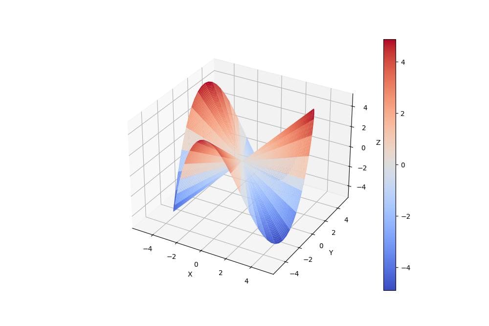
This code generates a 3D surface plot with a colorbar representing the z-values.

 

3D Polar Contour Plot

For a 3D polar contour plot, you can use the contourf function:

fig = plt.figure(figsize=(10, 8))
ax = fig.add_subplot(111, projection='3d')
r = np.linspace(0, 5, 50)
theta = np.linspace(0, 2 * np.pi, 100)
r, theta = np.meshgrid(r, theta)
z = r * np.cos(4 * theta)
contour = ax.contourf(r * np.cos(theta), r * np.sin(theta), z, cmap='viridis', levels=20)
fig.colorbar(contour)
ax.set_xlabel('X')
ax.set_ylabel('Y')
ax.set_zlabel('Z')
plt.show()

Output:

This code creates a 3D contour plot with filled contours representing the z-values.

 

Discontinuities in Polar Functions

To handle discontinuities in polar functions, you can use masked arrays:

import numpy.ma as ma
fig = plt.figure(figsize=(10, 8))
ax = fig.add_subplot(111, projection='3d')
r = np.linspace(0, 5, 100)
theta = np.linspace(0, 2 * np.pi, 200)
r, theta = np.meshgrid(r, theta)
z = np.tan(theta)
z_masked = ma.masked_where(np.abs(z) > 10, z)
surf = ax.plot_surface(r * np.cos(theta), r * np.sin(theta), z_masked, cmap='viridis')
fig.colorbar(surf)
ax.set_xlabel('X')
ax.set_ylabel('Y')
ax.set_zlabel('Z')
plt.show()

Output:

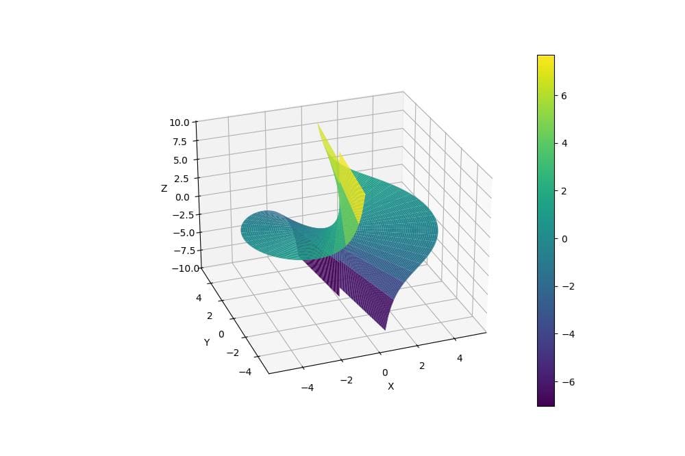
This code masks values where the tangent function approaches infinity.

 

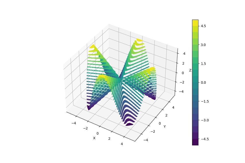
Plot Periodic Functions

To plot periodic functions, ensure your theta range covers multiple periods:

fig = plt.figure(figsize=(10, 8))
ax = fig.add_subplot(111, projection='3d')
r = np.linspace(0, 5, 50)
theta = np.linspace(0, 4 * np.pi, 200)
r, theta = np.meshgrid(r, theta)
z = r * np.sin(3 * theta)
surf = ax.plot_surface(r * np.cos(theta), r * np.sin(theta), z, cmap='coolwarm')
fig.colorbar(surf)
ax.set_xlabel('X')
ax.set_ylabel('Y')
ax.set_zlabel('Z')
plt.show()

Output:

This code plots a periodic function over multiple cycles that shows its repeating nature in 3D space.