Create 3D Plots Using IPyvolume in Jupyter Notebooks

IPyvolume is a powerful Python library for creating interactive 3D plots in Jupyter Notebooks.

This tutorial will guide you through creating various types of 3D plots using IPyvolume, from simple scatter plots to complex volume renderings.

To get started, install IPyvolume and import the necessary libraries:

!pip install ipyvolume
import ipyvolume as ipv
import numpy as np

 

 

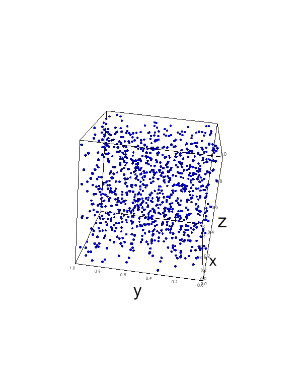
Scatter Plot

To create a 3D scatter plot, use the ipv.scatter() function:

x = np.random.random(1000)
y = np.random.random(1000)
z = np.random.random(1000)
fig = ipv.figure()
ipv.scatter(x, y, z, marker='sphere')
ipv.show()

Output:

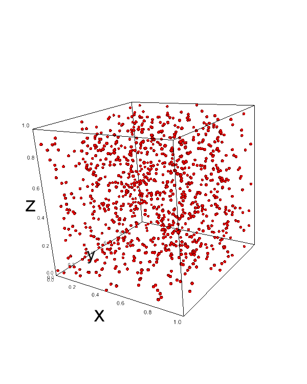
This code generates a 3D scatter plot with 1000 randomly distributed points.

The marker='sphere' parameter sets the point style to spheres.

 

Line Plot

To create a 3D line plot, you can use the ipv.plot() function:

t = np.linspace(0, 10, 1000)
x = np.cos(t)
y = np.sin(t)
z = t
fig = ipv.figure()
ipv.plot(x, y, z)
ipv.show()

Output:

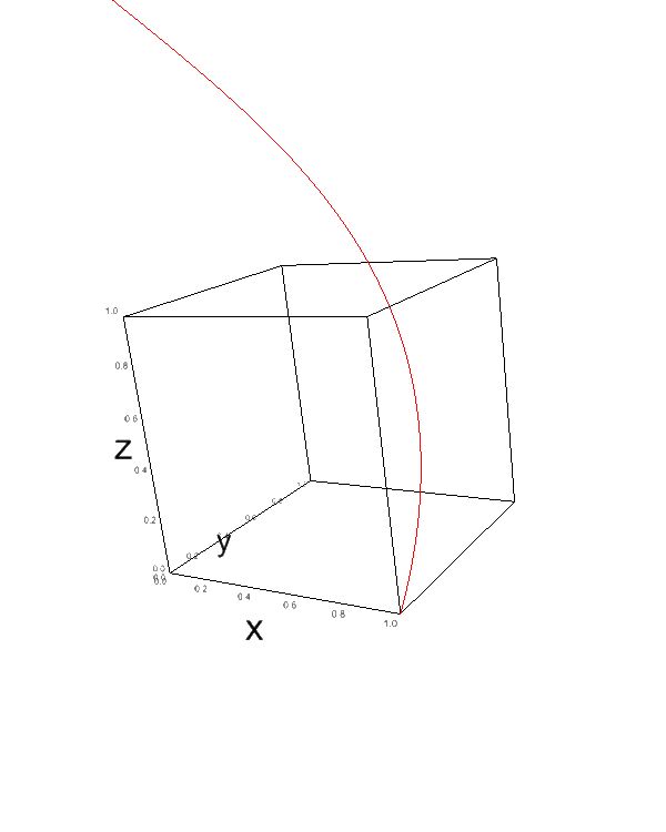
This code produces a 3D spiral line plot.

The t variable represents time, and x, y, and z are parametric equations for the spiral.

 

Surface Plot

To create a 3D surface plot, use the ipv.plot_surface() function:

x = np.linspace(-5, 5, 100)
y = np.linspace(-5, 5, 100)
x, y = np.meshgrid(x, y)
z = np.sin(np.sqrt(x**2 + y**2))
fig = ipv.figure()
ipv.plot_surface(x, y, z, color='orange')
ipv.show()

Output:

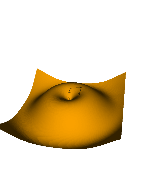
This code creates a 3D surface plot of a sinc function.

The np.meshgrid() function generates a 2D grid of x and y values, and z is calculated using these values.

 

Wireframe Plot

To create a wireframe plot, use the ipv.plot_wireframe() function:

x = np.linspace(-5, 5, 50)
y = np.linspace(-5, 5, 50)
x, y = np.meshgrid(x, y)
z = np.sin(np.sqrt(x**2 + y**2))
fig = ipv.figure()
ipv.plot_wireframe(x, y, z)
ipv.show()

Output:

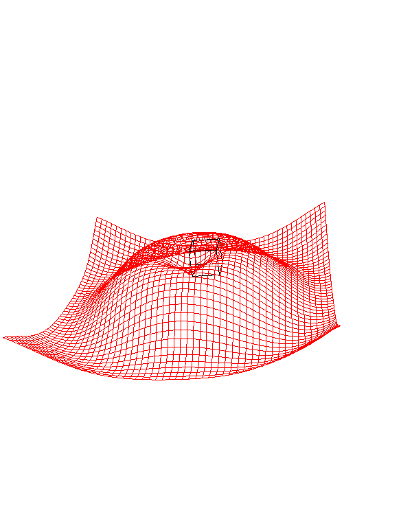
This code generates a wireframe representation of the same sinc function used in the surface plot example.

 

Quiver Plot (Vector Fields)

To create a quiver plot for visualizing vector fields, use the ipv.quiver() function:

x, y, z = np.meshgrid(np.arange(-2, 2, 0.5),
                      np.arange(-2, 2, 0.5),
                      np.arange(-2, 2, 0.5))

u = -1 - x**2 + y
v = 1 + x - y**2
w = 1 - z + y
fig = ipv.figure()
ipv.quiver(x, y, z, u, v, w)
ipv.show()

Output:

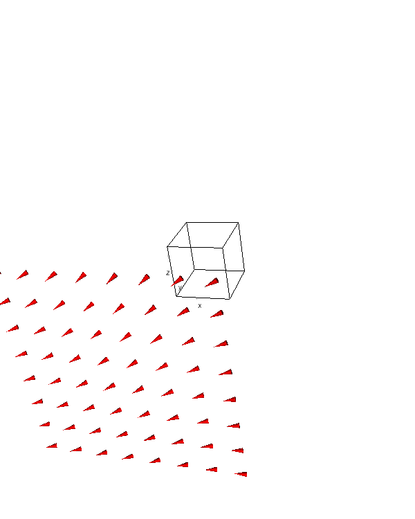
This code creates a 3D quiver plot representing a vector field. The u, v, and w variables define the vector components at each point in the 3D space.

 

Customize Plot Appearance

Change Colors and Colormaps

You can modify the color of your plots using the color parameter:

x, y, z = np.random.random((3, 1000))
c = x + y + z
fig = ipv.figure()
ipv.scatter(x, y, z, c=c, marker='sphere', size=2, color='blue')
ipv.show()

Output:

Customize Marker Types and Sizes

You can change the marker type and size in scatter plots using markerand size parameters:

x, y, z = np.random.random((3, 100))
fig = ipv.figure()
ipv.scatter(x, y, z, marker='sphere', size=2, color='red')
ipv.scatter(x + 0.5, y + 0.5, z + 0.5, marker='box', size=4, color='blue')
ipv.show()

Output:

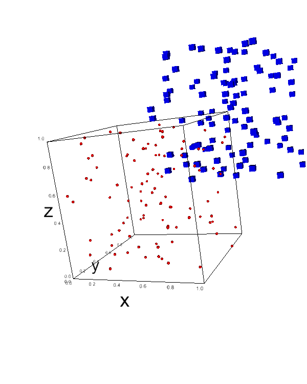
This code creates two scatter plots with different marker types (spheres and boxes) and sizes.