Create 3D Mesh Plots in Python using Matplotlib

In this tutorial, you’ll learn how to create various 3D mesh plots using Matplotlib, from simple triangular meshes to complex mathematical surfaces.

We’ll discover how to plot surfaces like Mobius strips and Klein bottles.

 

 

Triangular Mesh Plot

To create a basic triangular mesh plot, you can use the plot_trisurf() function:

import numpy as np
import matplotlib.pyplot as plt
x = np.random.rand(100)
y = np.random.rand(100)
z = np.sin(x*y)
fig = plt.figure(figsize=(10, 8))
ax = fig.add_subplot(111, projection='3d')
ax.plot_trisurf(x, y, z, cmap='viridis')
plt.show()

Output:

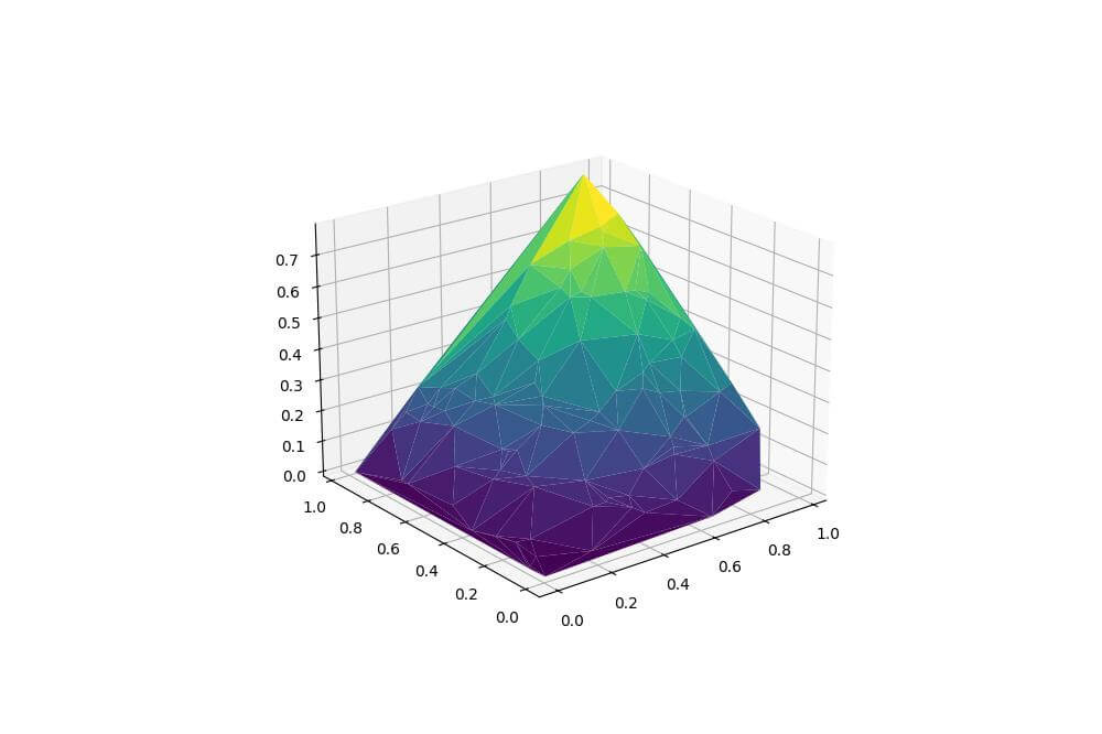
This code generates a 3D surface plot using randomly generated x and y coordinates, with z values calculated as the sine of their product.

 

Mobius Strip Plot

To visualize a Mobius strip, use parametric equations and plot_surface():

import numpy as np
import matplotlib.pyplot as plt
u = np.linspace(0, 2*np.pi, 100)
v = np.linspace(-1, 1, 25)
u, v = np.meshgrid(u, v)
x = (1 + 0.5*v*np.cos(u/2))*np.cos(u)
y = (1 + 0.5*v*np.cos(u/2))*np.sin(u)
z = 0.5*v*np.sin(u/2)
fig = plt.figure(figsize=(10, 8))
ax = fig.add_subplot(111, projection='3d')
ax.plot_surface(x, y, z, cmap='coolwarm')
plt.show()

Output:

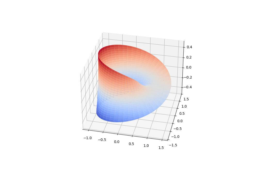
This code generates a Mobius strip, a surface with only one side and one boundary.

 

Klein Bottle Visualization

You can create a Klein bottle visualization using parametric equations:

import numpy as np
import matplotlib.pyplot as plt
u = np.linspace(0, 2*np.pi, 100)
v = np.linspace(0, 2*np.pi, 100)
u, v = np.meshgrid(u, v)
x = (2 + np.cos(v/2)*np.sin(u) - np.sin(v/2)*np.sin(2*u))*np.cos(v)
y = (2 + np.cos(v/2)*np.sin(u) - np.sin(v/2)*np.sin(2*u))*np.sin(v)
z = np.sin(v/2)*np.sin(u) + np.cos(v/2)*np.sin(2*u)
fig = plt.figure(figsize=(10, 8))
ax = fig.add_subplot(111, projection='3d')
ax.plot_surface(x, y, z, cmap='viridis', alpha=0.7)
plt.show()

Output:

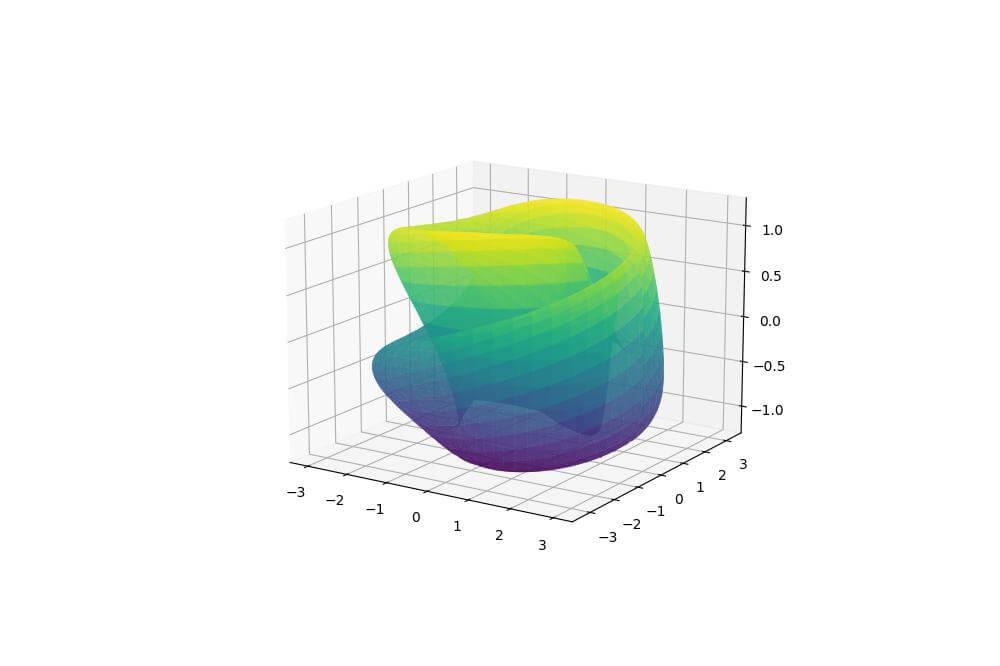
This code creates a 3D representation of a Klein bottle, a non-orientable surface that doesn’t have an inside or outside.

 

Sphere with Custom Coloring

You can create a sphere with custom coloring using plot_surface():

import numpy as np
import matplotlib.pyplot as plt
phi = np.linspace(0, np.pi, 100)
theta = np.linspace(0, 2*np.pi, 100)
x = np.outer(np.sin(theta), np.cos(phi))
y = np.outer(np.sin(theta), np.sin(phi))
z = np.outer(np.cos(theta), np.ones_like(phi))
fig = plt.figure(figsize=(10, 8))
ax = fig.add_subplot(111, projection='3d')
ax.plot_surface(x, y, z, facecolors=plt.cm.jet(z))
plt.show()

Output:

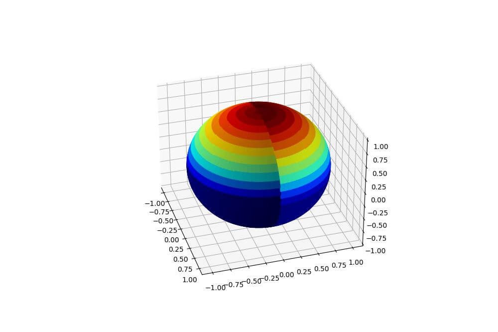
This code generates a sphere with custom coloring based on the z-coordinate.

The resulting plot displays a vibrant sphere with colors transitioning from blue at the bottom to red at the top.

 

Torus Plot

You can create a torus plot using parametric equations:

import numpy as np
import matplotlib.pyplot as plt
R, r = 5, 2
u = np.linspace(0, 2*np.pi, 100)
v = np.linspace(0, 2*np.pi, 100)
u, v = np.meshgrid(u, v)
x = (R + r*np.cos(v)) * np.cos(u)
y = (R + r*np.cos(v)) * np.sin(u)
z = r * np.sin(v)
fig = plt.figure(figsize=(10, 8))
ax = fig.add_subplot(111, projection='3d')
ax.plot_surface(x, y, z, cmap='plasma')
plt.show()

Output:

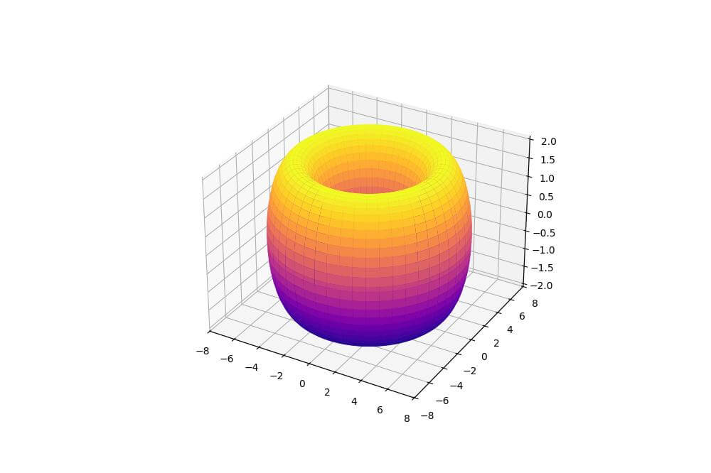
This code generates a torus with a donut-shaped surface.

The resulting plot shows the distinctive shape of the torus with a smooth color gradient.

 

Saddle Surface Plot

Visualize a saddle surface using the plot_surface() function:

import numpy as np
import matplotlib.pyplot as plt
x = np.linspace(-5, 5, 100)
y = np.linspace(-5, 5, 100)
x, y = np.meshgrid(x, y)
z = x**2 - y**2
fig = plt.figure(figsize=(10, 8))
ax = fig.add_subplot(111, projection='3d')
ax.plot_surface(x, y, z, cmap='coolwarm')
plt.show()

Output:

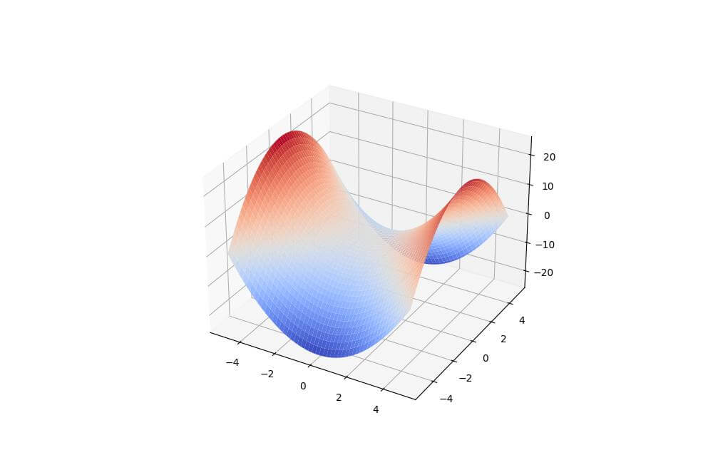
This code creates a saddle surface, which has a distinctive shape that curves up in one direction and down in the perpendicular direction.

The resulting plot shows the saddle-like curvature of the surface.

 

Enneper Surface Plot

You can visualize an Enneper surface using parametric equations:

import numpy as np
import matplotlib.pyplot as plt
u = np.linspace(-2, 2, 100)
v = np.linspace(-2, 2, 100)
u, v = np.meshgrid(u, v)
x = u - u**3/3 + u*v**2
y = v - v**3/3 + v*u**2
z = u**2 - v**2
fig = plt.figure(figsize=(10, 8))
ax = fig.add_subplot(111, projection='3d')
ax.plot_surface(x, y, z, cmap='coolwarm')
plt.show()

Output:

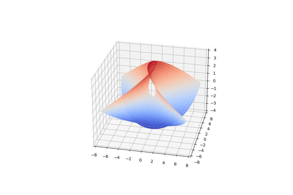
This code generates an Enneper surface with a self-intersecting minimal surface.

The resulting plot shows the complex, twisted nature of the Enneper surface with its characteristic shape.

 

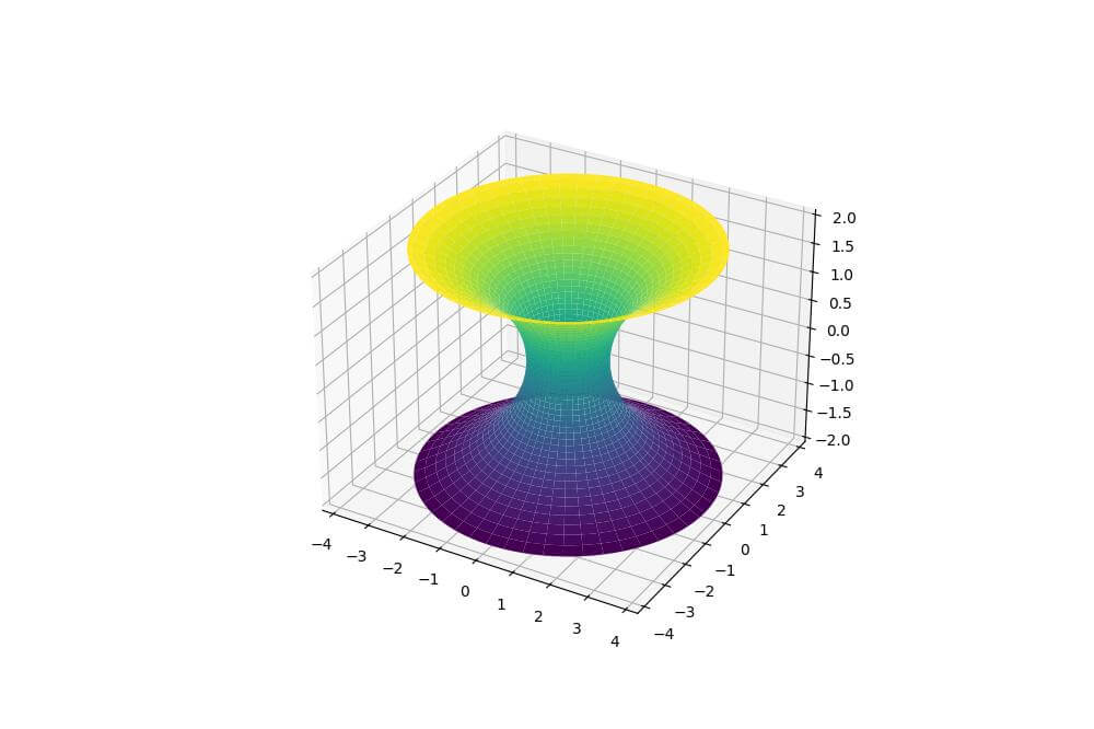
Catenoid Surface Plot

You can create a catenoid surface using hyperbolic cosine function by rotating a catenary curve around an axis:

import numpy as np
import matplotlib.pyplot as plt
u = np.linspace(-2, 2, 100)
v = np.linspace(0, 2*np.pi, 100)
u, v = np.meshgrid(u, v)
x = np.cosh(u) * np.cos(v)
y = np.cosh(u) * np.sin(v)
z = u
fig = plt.figure(figsize=(10, 8))
ax = fig.add_subplot(111, projection='3d')
ax.plot_surface(x, y, z, cmap='viridis')
plt.show()

Output:

 

Helicoid Surface Plot

You can visualize a helicoid surface using parametric equations:

import numpy as np
import matplotlib.pyplot as plt
u = np.linspace(-10, 10, 100)
v = np.linspace(-np.pi, np.pi, 100)
u, v = np.meshgrid(u, v)
x = u * np.cos(v)
y = u * np.sin(v)
z = v
fig = plt.figure(figsize=(10, 8))
ax = fig.add_subplot(111, projection='3d')
ax.plot_surface(x, y, z, cmap='plasma')
plt.show()

Output:

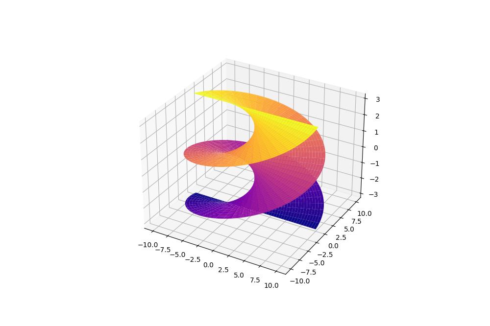
This code creates a helicoid, a ruled surface that resembles a screw or a spiral staircase.