How to Plot 3D Cones in Python using Matplotlib

In this tutorial, you’ll learn how to create various 3D cone plots using Matplotlib in Python.

You’ll start with a basic cone plot and then add more complex features like wireframes, multiple cones, transparency, gradient colors, and unique shapes.

 

 

Basic 3D Cone Plot

To create a basic 3D cone plot, you’ll use Matplotlib mplot3d toolkit:

import numpy as np
import matplotlib.pyplot as plt
from mpl_toolkits.mplot3d import Axes3D
fig = plt.figure(figsize=(10, 8))
ax = fig.add_subplot(111, projection='3d')
r = np.linspace(0, 1, 100)
theta = np.linspace(0, 2*np.pi, 100)
r, theta = np.meshgrid(r, theta)
x = r * np.cos(theta)
y = r * np.sin(theta)
z = r
ax.plot_surface(x, y, z, cmap='viridis')
ax.set_xlabel('X')
ax.set_ylabel('Y')
ax.set_zlabel('Z')
ax.set_title('Basic 3D Cone')
plt.show()

Output:

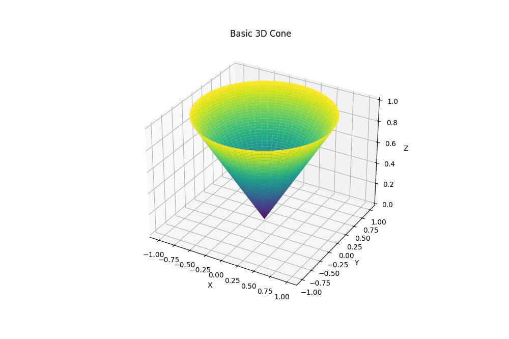
The cone is centered at the origin and extends along the z-axis.

The plot_surface function creates the 3D surface of the cone.

 

3D Cone with Wireframe

You can add a wireframe to your 3D cone to highlight its structure:

import numpy as np
import matplotlib.pyplot as plt
from mpl_toolkits.mplot3d import Axes3D
fig = plt.figure(figsize=(10, 8))
ax = fig.add_subplot(111, projection='3d')
r = np.linspace(0, 1, 20)
theta = np.linspace(0, 2*np.pi, 40)
r, theta = np.meshgrid(r, theta)
x = r * np.cos(theta)
y = r * np.sin(theta)
z = r
ax.plot_surface(x, y, z, alpha=0.8, cmap='coolwarm')
ax.plot_wireframe(x, y, z, color='black', linewidth=0.5)
ax.set_xlabel('X')
ax.set_ylabel('Y')
ax.set_zlabel('Z')
ax.set_title('3D Cone with Wireframe')
plt.show()

Output:

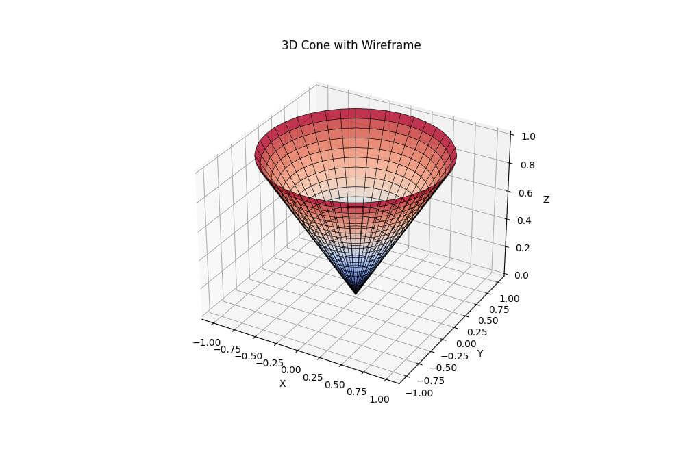
The alpha parameter in plot_surface makes the surface slightly transparent.

The wireframe is plotted in black with a thin line width.

 

Multiple 3D Cones

To plot multiple 3D cones, you can create separate cone data and plot them on the same axis:

import numpy as np
import matplotlib.pyplot as plt
from mpl_toolkits.mplot3d import Axes3D
fig = plt.figure(figsize=(12, 10))
ax = fig.add_subplot(111, projection='3d')
def plot_cone(ax, x_center, y_center, z_base, height, radius, color):
    r = np.linspace(0, radius, 20)
    theta = np.linspace(0, 2*np.pi, 40)
    r, theta = np.meshgrid(r, theta)
    x = r * np.cos(theta) + x_center
    y = r * np.sin(theta) + y_center
    z = z_base + (height / radius) * r
    ax.plot_surface(x, y, z, color=color, alpha=0.7)
plot_cone(ax, 0, 0, 0, 1, 1, 'red')
plot_cone(ax, 2, 2, 0, 1.5, 0.8, 'blue')
plot_cone(ax, -2, -2, 0, 0.8, 1.2, 'green')
ax.set_xlabel('X')
ax.set_ylabel('Y')
ax.set_zlabel('Z')
ax.set_title('Multiple 3D Cones')
plt.show()

Output:

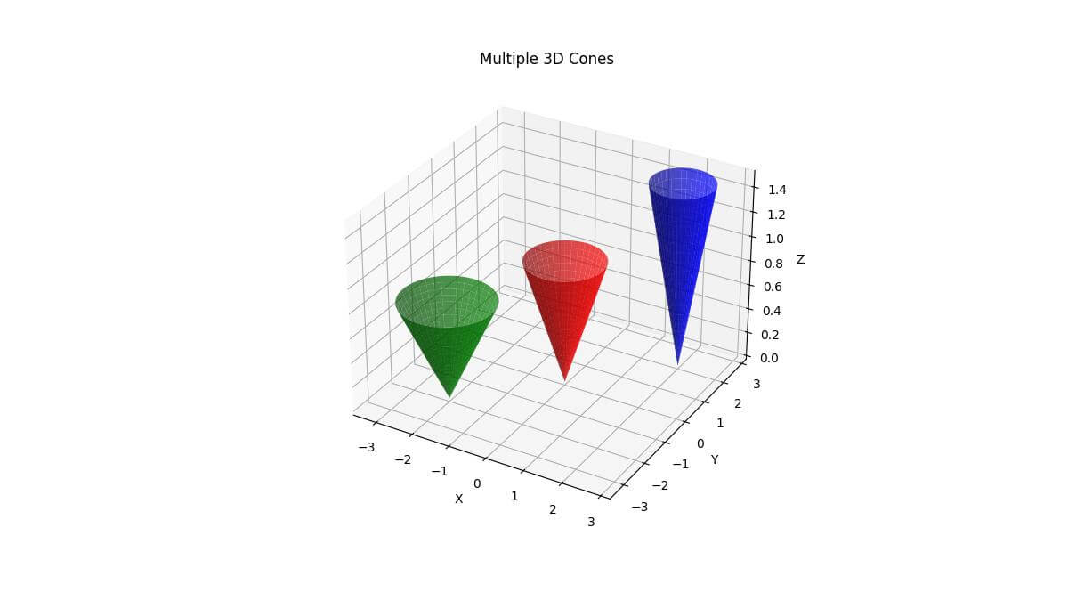
This code plots three cones with different positions, heights, radii, and colors.

The alpha parameter is used to make the cones slightly transparent so you can see overlapping areas.

 

3D Cone with Mesh Only

To create a 3D cone with only the mesh visible, you can use the plot_wireframe function:

import numpy as np
import matplotlib.pyplot as plt
from mpl_toolkits.mplot3d import Axes3D
fig = plt.figure(figsize=(10, 8))
ax = fig.add_subplot(111, projection='3d')
r = np.linspace(0, 1, 20)
theta = np.linspace(0, 2*np.pi, 40)
r, theta = np.meshgrid(r, theta)
x = r * np.cos(theta)
y = r * np.sin(theta)
z = r
ax.plot_wireframe(x, y, z, color='magenta', linewidth=1)
ax.set_xlabel('X')
ax.set_ylabel('Y')
ax.set_zlabel('Z')
ax.set_title('3D Cone with Mesh Only')
plt.show()

Output:

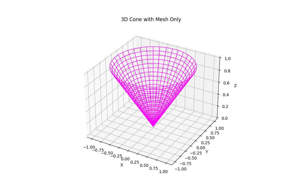
The plot_wireframe function is used instead of plot_surface.

 

3D Oblique Cone

To create an oblique cone, you can modify the z-coordinate calculation:

import numpy as np
import matplotlib.pyplot as plt
from mpl_toolkits.mplot3d import Axes3D
fig = plt.figure(figsize=(10, 8))
ax = fig.add_subplot(111, projection='3d')
r = np.linspace(0, 1, 100)
theta = np.linspace(0, 2*np.pi, 100)
r, theta = np.meshgrid(r, theta)
x = r * np.cos(theta)
y = r * np.sin(theta)
z = r + 0.5 * x  # Adding x component to make it oblique
surf = ax.plot_surface(x, y, z, cmap='viridis', linewidth=0, antialiased=False)
ax.set_xlabel('X')
ax.set_ylabel('Y')
ax.set_zlabel('Z')
ax.set_title('3D Oblique Cone')
fig.colorbar(surf, shrink=0.5, aspect=5)
plt.show()

Output:

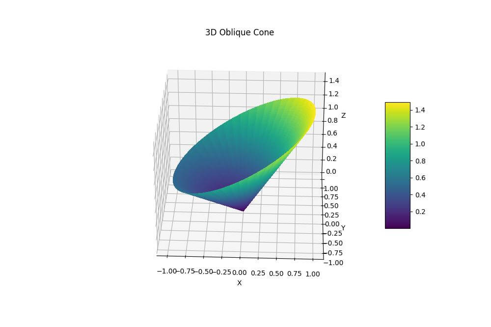
This code creates an oblique cone by adding an x-component to the z-coordinate calculation.

 

3D Double Cone

You can create a double cone by extending the z-axis in both positive and negative directions:

import numpy as np
import matplotlib.pyplot as plt
from mpl_toolkits.mplot3d import Axes3D
fig = plt.figure(figsize=(10, 8))
ax = fig.add_subplot(111, projection='3d')

# Generate data for the double cone
theta = np.linspace(0, 2*np.pi, 100)
z = np.linspace(-1, 1, 100)
theta, z = np.meshgrid(theta, z)
r = np.abs(z)
x = r * np.cos(theta)
y = r * np.sin(theta)
ax.plot_surface(x, y, z, cmap='viridis')
ax.set_xlabel('X')
ax.set_ylabel('Y')
ax.set_zlabel('Z')
ax.set_title('3D Double Cone')
plt.show()

Output:

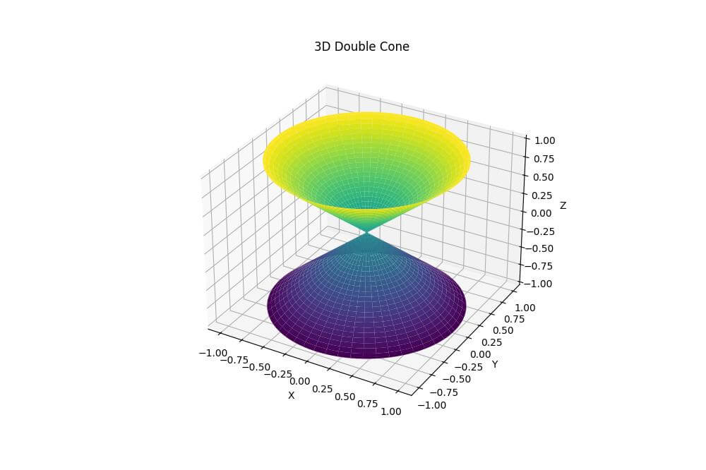
This code creates a double cone by extending the z-coordinate in both positive and negative directions.

The x and y coordinates are duplicated to match the extended z-coordinate.

 

3D Double Cone with Common Base Shift

To create a double cone with a shifted common base, you can modify the z-coordinate calculation:

import numpy as np
import matplotlib.pyplot as plt
from mpl_toolkits.mplot3d import Axes3D
fig = plt.figure(figsize=(10, 8))
ax = fig.add_subplot(111, projection='3d')
radius = 1  # Base radius of the cones
height = 2  # Height of each cone
shift = 0.5  # Shift amount for the common base
theta = np.linspace(0, 2*np.pi, 100)
z = np.linspace(-height, height, 100)
theta, z = np.meshgrid(theta, z)
x = radius * (1 - np.abs(z) / height) * np.cos(theta)
y = radius * (1 - np.abs(z) / height) * np.sin(theta)

# Modify z-coordinate calculation for shifted common base
z_shifted = np.where(z >= 0, z + shift, z - shift)
ax.plot_surface(x, y, z_shifted, cmap='viridis')
ax.set_xlabel('X')
ax.set_ylabel('Y')
ax.set_zlabel('Z')
ax.set_title('Double Cone with Shifted Common Base')
plt.show()

Output:

The z-coordinate calculation is modified to move the common base to z=0.5.