Create 3D Ball Trajectory Plot in Python

In this tutorial, you’ll learn how to create a 3D ball trajectory plot in Python.

We’ll start with basic physics equations and gradually add complexity, such as air resistance and spin.

 

 

Calculate the Trajectory

To calculate the trajectory, use the basic equations of motion. These equations describe the position of the ball in three dimensions over time.

import numpy as np
g = 9.81  # Acceleration due to gravity (m/s^2)
v0 = 20  # Initial velocity (m/s)
angle = 45  # Launch angle (degrees)
angle_rad = np.radians(angle)  # Convert angle to radians

# Initial velocity components
v0_x = v0 * np.cos(angle_rad)
v0_y = v0 * np.sin(angle_rad)
v0_z = 0  # No initial velocity in the z-direction

Output:

 

This code defines the initial conditions for the ball’s launch, including the initial velocity and angle.

It calculates the velocity components in the x and y directions using trigonometry.

You can create functions to calculate the position coordinates (x, y, z) based on time.

def position_x(t):
  return v0_x * t
def position_y(t):
  return v0_y * t - 0.5 * g * t**2
def position_z(t):
  return v0_z * t

These functions calculate the x, y, and z positions of the ball at any given time t.

The y-position includes the effect of gravity, which causes the ball to follow a parabolic path.

 

Generate Time Points

To calculate the trajectory, you can create an array of time points.

# Time of flight
t_flight = 2 * v0_y / g

# Time points
t_points = np.linspace(0, t_flight, num=500)

Here we calculate the total time of flight and generate an array of time points from 0 to the time of flight.

This array will be used to compute the position coordinates at each time step.

You can use the position functions to calculate the coordinates for each time point.

x_points = position_x(t_points)
y_points = position_y(t_points)
z_points = position_z(t_points)

This code uses the previously defined functions to calculate the x, y, and z coordinates for each time point in the trajectory.

 

Simple Parabolic Trajectory

Let’s plot the simple parabolic trajectory using Matplotlib:

import matplotlib.pyplot as plt
from mpl_toolkits.mplot3d import Axes3D
fig = plt.figure()
ax = fig.add_subplot(111, projection='3d')
ax.plot(x_points, y_points, z_points, label='Parabolic Trajectory')
ax.set_xlabel('X Position (m)')
ax.set_ylabel('Y Position (m)')
ax.set_zlabel('Z Position (m)')
ax.legend()
plt.show()

Output:

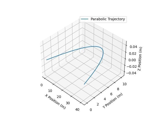
The plot shows the ball’s path in three dimensions, with labels for each axis.

 

With Air Resistance

Let’s modify the trajectory to include air resistance:

C_d = 0.47  # Drag coefficient for a sphere
rho = 1.225  # Air density (kg/m^3)
A = 0.045  # Cross-sectional area (m^2)
m = 0.145  # Mass of the ball (kg)
def position_with_drag(t, dt=0.01):
    x, y, z = 0, 0, 0
    vx, vy, vz = v0_x, v0_y, v0_z
    x_points, y_points, z_points = [x], [y], [z]  
    for _ in np.arange(0, t, dt):
        v = np.sqrt(vx**2 + vy**2 + vz**2)
        F_d = 0.5 * C_d * rho * A * v**2
        ax = -F_d * vx / (m * v)
        ay = -g - (F_d * vy / (m * v))
        az = -F_d * vz / (m * v)      
        vx += ax * dt
        vy += ay * dt
        vz += az * dt      
        x += vx * dt
        y += vy * dt
        z += vz * dt      
        x_points.append(x)
        y_points.append(y)
        z_points.append(z)  
    return np.array(x_points), np.array(y_points), np.array(z_points)
x_drag, y_drag, z_drag = position_with_drag(t_flight)
import matplotlib.pyplot as plt
from mpl_toolkits.mplot3d import Axes3D
fig = plt.figure()
ax = fig.add_subplot(111, projection='3d')
ax.plot(x_drag, y_drag, z_drag, label='Trajectory with air resistance')
ax.set_xlabel('X Position (m)')
ax.set_ylabel('Y Position (m)')
ax.set_zlabel('Z Position (m)')
ax.legend()
plt.show()

Output:

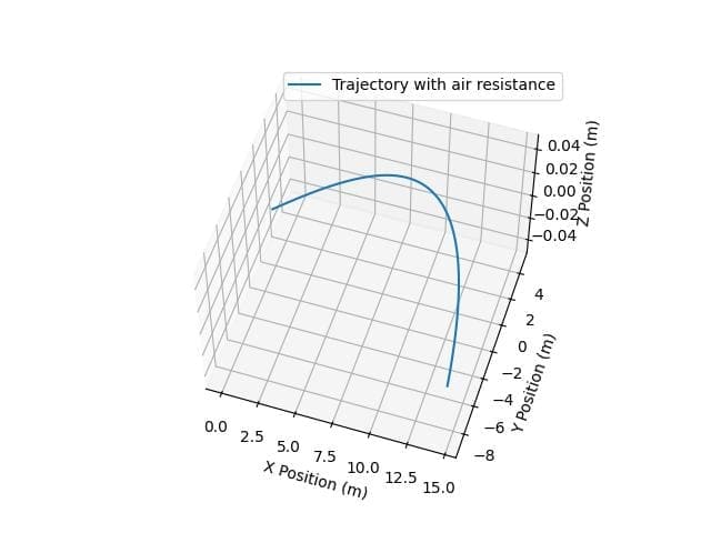
This code simulates the ball’s trajectory with air resistance by iteratively updating the position and velocity.

It accounts for the drag force, which depends on the velocity and other factors.

 

With Spin

You can include the Magnus effect to simulate the effect of spin on the trajectory.

omega = 50  # Spin rate (rad/s)
S = 0.00041  # Magnus coefficient
def position_with_spin(t, dt=0.01):
    x, y, z = 0, 0, 0
    vx, vy, vz = v0_x, v0_y, v0_z
    x_points, y_points, z_points = [x], [y], [z]  
    for _ in np.arange(0, t, dt):
        v = np.sqrt(vx**2 + vy**2 + vz**2)
        F_d = 0.5 * C_d * rho * A * v**2
        F_m = S * omega * v
        ax = (-F_d * vx + F_m * vy) / (m * v)
        ay = -g - (F_d * vy - F_m * vx) / (m * v)
        az = -F_d * vz / (m * v)      
        vx += ax * dt
        vy += ay * dt
        vz += az * dt      
        x += vx * dt
        y += vy * dt
        z += vz * dt
        x_points.append(x)
        y_points.append(y)
        z_points.append(z)  
    return np.array(x_points), np.array(y_points), np.array(z_points)
x_spin, y_spin, z_spin = position_with_spin(t_flight)
import matplotlib.pyplot as plt
from mpl_toolkits.mplot3d import Axes3D
fig = plt.figure()
ax = fig.add_subplot(111, projection='3d')
ax.plot(x_spin, y_spin, z_spin, label='Trajectory With Spin')
ax.set_xlabel('X Position (m)')
ax.set_ylabel('Y Position (m)')
ax.set_zlabel('Z Position (m)')
ax.legend()
plt.show()

Output:

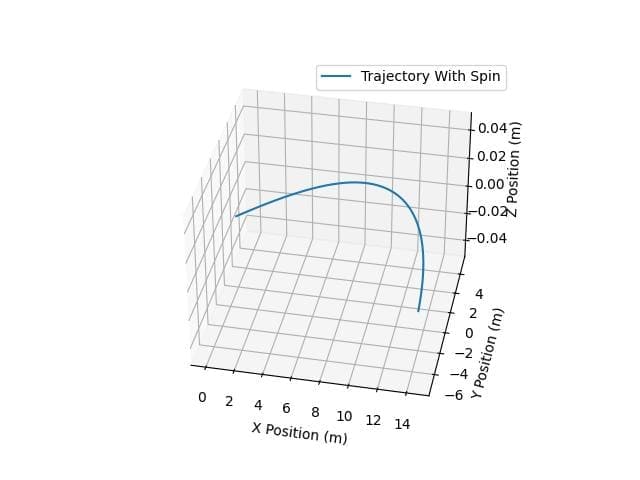
This code simulates the ball’s trajectory with the Magnus effect, which causes the ball to curve due to spin. The Magnus force is added to the equations of motion.

 

Compare Trajectories With Different Velocities

Plot trajectories with different initial velocities.

velocities = [10, 20, 30]
colors = ['r', 'g', 'b']
fig = plt.figure()
ax = fig.add_subplot(111, projection='3d')
for v0, color in zip(velocities, colors):
  v0_x = v0 * np.cos(angle_rad)
  v0_y = v0 * np.sin(angle_rad)
  x_points, y_points, z_points = position_with_drag(t_flight)
  ax.plot(x_points, y_points, z_points, color=color, label=f'v0 = {v0} m/s')
ax.set_xlabel('X Position (m)')
ax.set_ylabel('Y Position (m)')
ax.set_zlabel('Z Position (m)')
ax.legend()
plt.show()

Output:

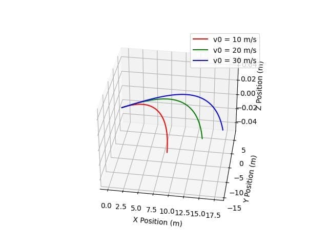
This code plots multiple trajectories with varying initial velocities on the same graph to compare how the initial speed affects the trajectory.

 

Compare Different Launch Angles

You can plot trajectories with different launch angles by assigning different angles:

angles = [30, 45, 60]
colors = ['r', 'g', 'b']
fig = plt.figure()
ax = fig.add_subplot(111, projection='3d')
for angle, color in zip(angles, colors):
  angle_rad = np.radians(angle)
  v0_x = v0 * np.cos(angle_rad)
  v0_y = v0 * np.sin(angle_rad)
  x_points, y_points, z_points = position_with_drag(t_flight)
  ax.plot(x_points, y_points, z_points, color=color, label=f'angle = {angle}°')
ax.set_xlabel('X Position (m)')
ax.set_ylabel('Y Position (m)')
ax.set_zlabel('Z Position (m)')
ax.legend()
plt.show()

Output:

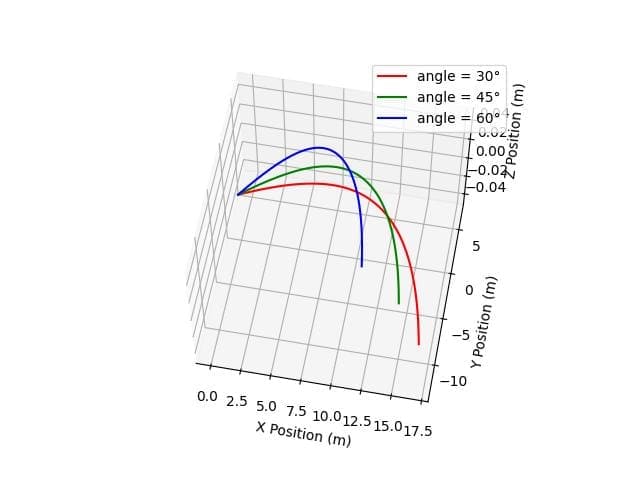
This code plots multiple trajectories with varying launch angles on the same graph to compare how the angle affects the trajectory.

 

Different Gravitational Strengths

You can simulate trajectories under different gravitational fields like this:

gravities = [9.81, 1.62]  # Earth and Moon gravity
labels = ['Earth', 'Moon']
colors = ['r', 'b']
fig = plt.figure()
ax = fig.add_subplot(111, projection='3d')
for g, label, color in zip(gravities, labels, colors):
  x_points, y_points, z_points = position_with_drag(t_flight)
  ax.plot(x_points, y_points, z_points, color=color, label=label)
ax.set_xlabel('X Position (m)')
ax.set_ylabel('Y Position (m)')
ax.set_zlabel('Z Position (m)')
ax.legend()
plt.show()

Output:

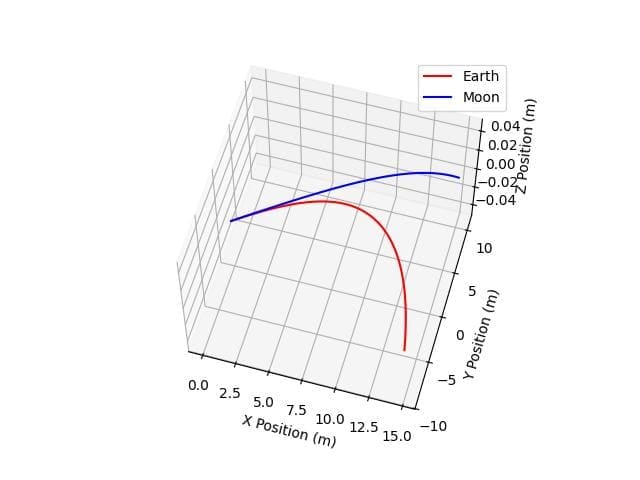
This code simulates and plots trajectories under different gravitational strengths, such as those on Earth and the Moon to show how gravity affects the trajectory.

 

Trajectories in Different Air Densities

You can simulate trajectories in different air densities like this:

densities = [1.225, 0.413]  # Sea level and high altitude
labels = ['Sea Level', 'High Altitude']
colors = ['r', 'b']
fig = plt.figure()
ax = fig.add_subplot(111, projection='3d')
for rho, label, color in zip(densities, labels, colors):
  x_points, y_points, z_points = position_with_drag(t_flight)
  ax.plot(x_points, y_points, z_points, color=color, label=label)
ax.set_xlabel('X Position (m)')
ax.set_ylabel('Y Position (m)')
ax.set_zlabel('Z Position (m)')
ax.legend()
plt.show()

Output:

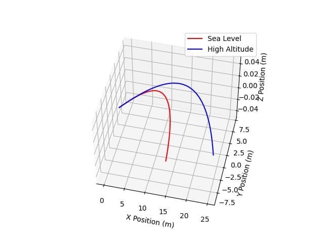
This code simulates and plots trajectories in different air densities, such as at sea level and high altitude, to show how air density affects the trajectory.