How to Smooth 3D Surface Plot in Python

In this tutorial, you’ll learn how to create smooth 3D surface plots in Python.

We’ll start with a basic plot and then explore various methods to enhance its smoothness.

 

 

To get started, import the required libraries and some sample data:

import numpy as np
import matplotlib.pyplot as plt
from mpl_toolkits.mplot3d import Axes3D
np.random.seed(42)
x = np.random.rand(100) * 4 - 2
y = np.random.rand(100) * 4 - 2
z = x**2 + y**2 + np.random.normal(0, 0.5, 100)

 

Using Interpolation

scipy griddata

To create a smoother surface, you can use interpolation methods. Let’s start with scipy griddata function:

from scipy.interpolate import griddata

# Create a grid of points
xi = yi = np.linspace(-2, 2, 100)
xi, yi = np.meshgrid(xi, yi)

# Interpolate the data onto the grid
zi = griddata((x, y), z, (xi, yi), method='cubic')

# Plot the interpolated surface
fig = plt.figure(figsize=(10, 8))
ax = fig.add_subplot(111, projection='3d')
surf = ax.plot_surface(xi, yi, zi, cmap='viridis')
ax.set_xlabel('X')
ax.set_ylabel('Y')
ax.set_zlabel('Z')
plt.title('Smooth 3D Surface Plot using griddata')
fig.colorbar(surf)
plt.show()

Output:

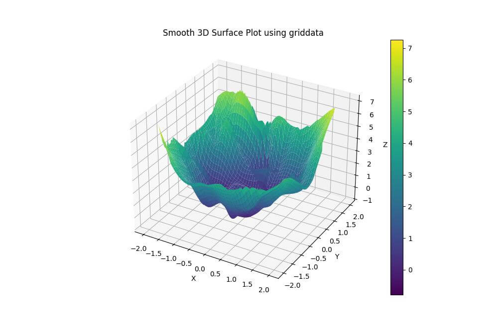
The griddata function interpolates the scattered data onto a regular grid, creating a continuous surface.

The ‘cubic’ method provides a smoother result compared to linear interpolation.

LinearNDInterpolator

We can use LinearNDInterpolator to interpolate the scattered data:

import numpy as np
import matplotlib.pyplot as plt
from mpl_toolkits.mplot3d import Axes3D
from scipy.interpolate import LinearNDInterpolator

np.random.seed(42)
x = np.random.rand(100) * 4 - 2
y = np.random.rand(100) * 4 - 2
z = x**2 + y**2 + np.random.normal(0, 0.5, 100)
fig = plt.figure(figsize=(10, 8))
ax = fig.add_subplot(111, projection='3d')
ax.scatter(x, y, z, c='r', marker='o', label='Data Points')

# Create an interpolation function using LinearNDInterpolator
interp_func = LinearNDInterpolator(list(zip(x, y)), z)
xi = yi = np.linspace(-2, 2, 100)
xi, yi = np.meshgrid(xi, yi)
zi = interp_func(xi, yi)
surf = ax.plot_surface(xi, yi, zi, cmap='viridis', alpha=0.7)
ax.set_xlabel('X')
ax.set_ylabel('Y')
ax.set_zlabel('Z')
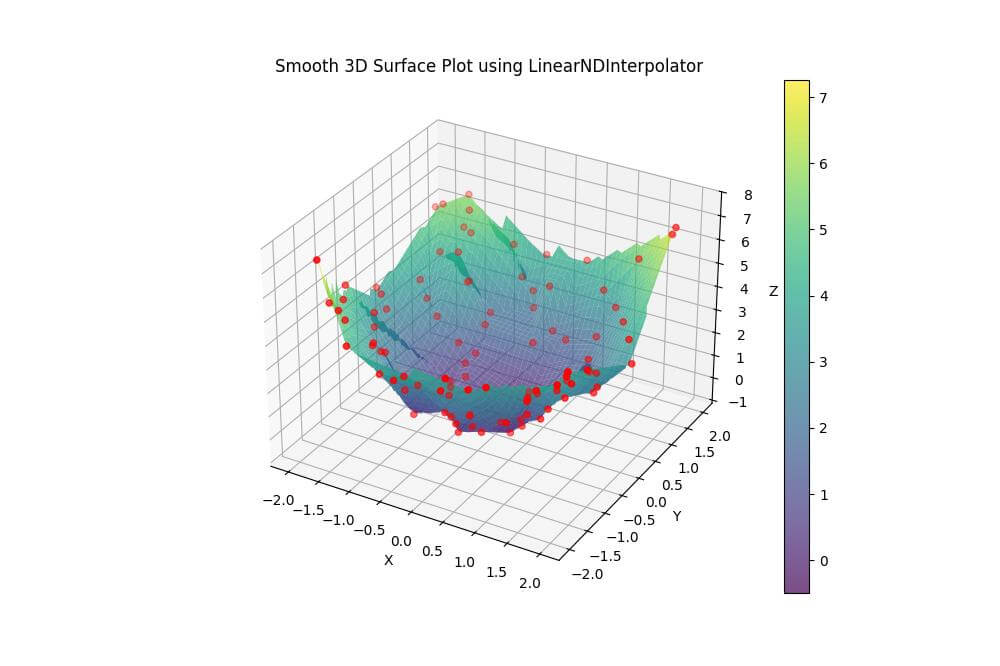
plt.title('Smooth 3D Surface Plot using LinearNDInterpolator')
fig.colorbar(surf)
plt.show()

Output:

 

Using Filtering

Gaussian filter

You can apply filters to smooth the interpolated surface. Let’s start with a Gaussian filter:

from scipy.ndimage import gaussian_filter

# Apply Gaussian filter to the interpolated data
zi_smooth = gaussian_filter(zi, sigma=2)

# Plot the smoothed surface
fig = plt.figure(figsize=(10, 8))
ax = fig.add_subplot(111, projection='3d')
surf = ax.plot_surface(xi, yi, zi_smooth, cmap='viridis')
ax.set_xlabel('X')
ax.set_ylabel('Y')
ax.set_zlabel('Z')
plt.title('Smooth 3D Surface Plot using Gaussian Filter')
fig.colorbar(surf)
plt.show()

Output:

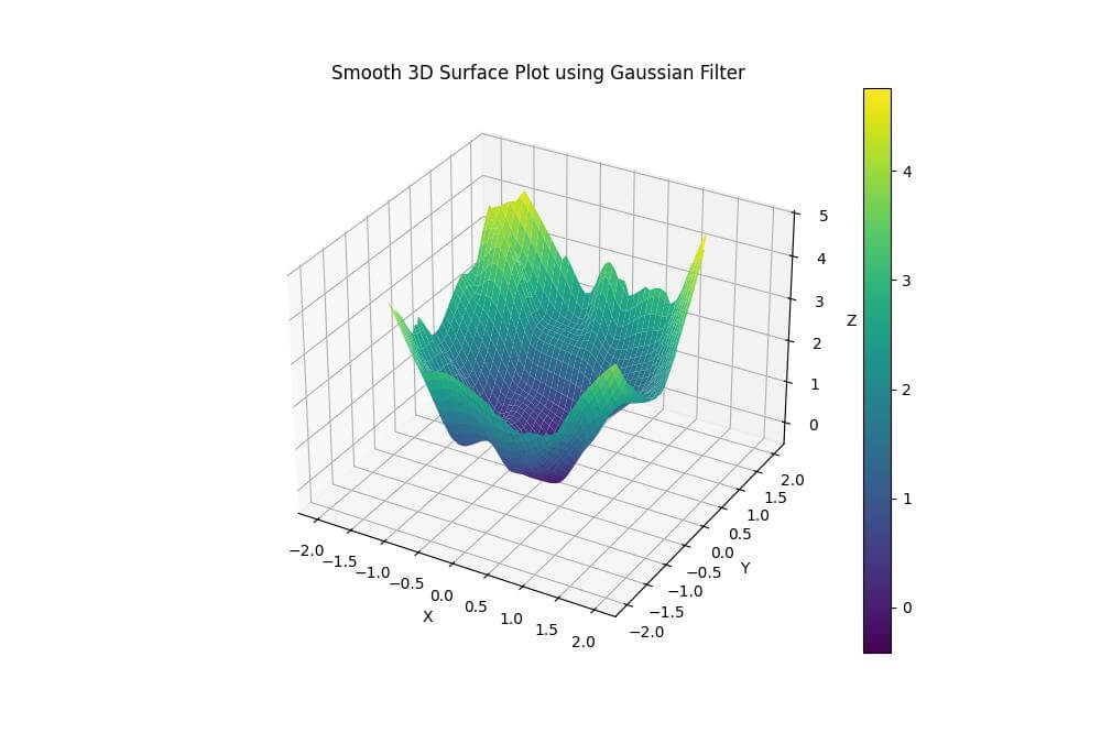
The Gaussian filter reduces noise and smooths out small variations in the surface.

Median filter

For a different smoothing effect, you can use a median filter:

from scipy.ndimage import median_filter

# Apply median filter to the interpolated data
zi_smooth = median_filter(zi, size=5)

# Plot the smoothed surface
fig = plt.figure(figsize=(10, 8))
ax = fig.add_subplot(111, projection='3d')
surf = ax.plot_surface(xi, yi, zi_smooth, cmap='viridis')
ax.set_xlabel('X')
ax.set_ylabel('Y')
ax.set_zlabel('Z')
plt.title('Smooth 3D Surface Plot using Median Filter')
fig.colorbar(surf)
plt.show()

Output:

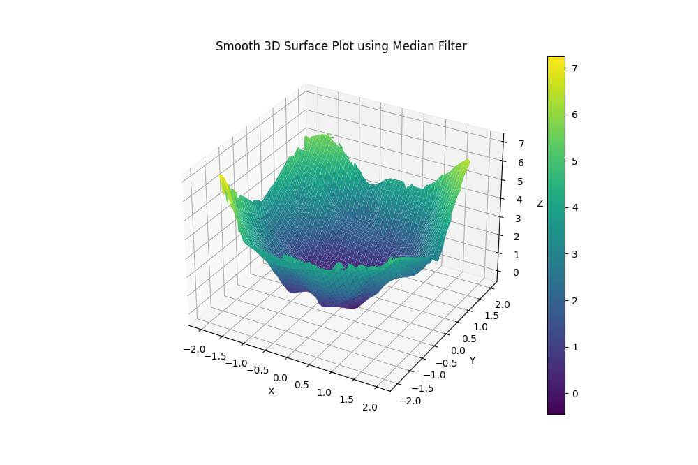
The median filter is effective at removing outliers and preserving edges in the data.

Savitzky-Golay filter

For more advanced smoothing, you can use the Savitzky-Golay filter:

from scipy.signal import savgol_filter

# Apply Savitzky-Golay filter to each row and column of the interpolated data
zi_smooth = savgol_filter(zi, window_length=15, polyorder=3, axis=0)
zi_smooth = savgol_filter(zi_smooth, window_length=15, polyorder=3, axis=1)

# Plot the smoothed surface
fig = plt.figure(figsize=(10, 8))
ax = fig.add_subplot(111, projection='3d')
surf = ax.plot_surface(xi, yi, zi_smooth, cmap='viridis')
ax.set_xlabel('X')
ax.set_ylabel('Y')
ax.set_zlabel('Z')
plt.title('Smooth 3D Surface Plot using Savitzky-Golay Filter')
fig.colorbar(surf)
plt.show()

Output:

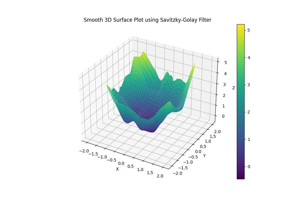
The Savitzky-Golay filter is useful for smoothing data with varying frequency content.

 

Mesh smoothing: Laplacian smoothing

For mesh-based smoothing, you can implement Laplacian smoothing:

def laplacian_smooth(vertices, iterations=5):
  for _ in range(iterations):
      new_vertices = np.zeros_like(vertices)
      for i in range(1, vertices.shape[0] - 1):
          for j in range(1, vertices.shape[1] - 1):
              new_vertices[i, j] = 0.25 * (vertices[i-1, j] + vertices[i+1, j] + 
                                           vertices[i, j-1] + vertices[i, j+1])
      vertices = new_vertices
  return vertices

# Apply Laplacian smoothing to the interpolated data
zi_smooth = laplacian_smooth(zi, iterations=10)

# Plot the smoothed surface
fig = plt.figure(figsize=(10, 8))
ax = fig.add_subplot(111, projection='3d')
surf = ax.plot_surface(xi, yi, zi_smooth, cmap='viridis')
ax.set_xlabel('X')
ax.set_ylabel('Y')
ax.set_zlabel('Z')
plt.title('Smooth 3D Surface Plot using Laplacian Smoothing')
fig.colorbar(surf)
plt.show()

Output:

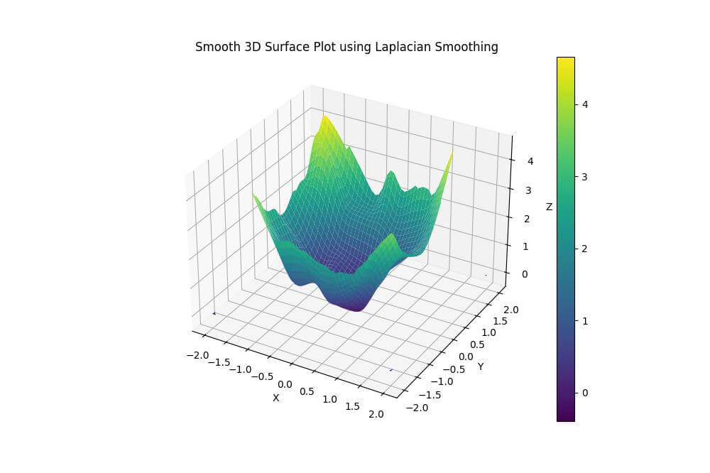
Laplacian smoothing iteratively adjusts each vertex position based on its neighbors.

 

Using Moving average

You can apply a moving average filter to smooth the surface:

def moving_average_2d(data, window_size):
  return np.convolve(data.ravel(), np.ones(window_size), mode='same').reshape(data.shape) / window_size

# Apply moving average filter to the interpolated data
zi_smooth = moving_average_2d(zi, 5)

# Plot the smoothed surface
fig = plt.figure(figsize=(10, 8))
ax = fig.add_subplot(111, projection='3d')
surf = ax.plot_surface(xi, yi, zi_smooth, cmap='viridis')
ax.set_xlabel('X')
ax.set_ylabel('Y')
ax.set_zlabel('Z')
plt.title('Smooth 3D Surface Plot using Moving Average')
fig.colorbar(surf)
plt.show()

Output:

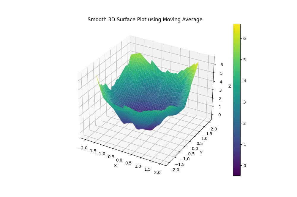
This method reduces local variations by averaging neighboring values.

 

Spline smoothing (Thin-plate splines)

Thin-plate splines offer another approach to create smooth surfaces:

from scipy.interpolate import Rbf
rbf = Rbf(x, y, z, function='thin_plate', smooth=0.1)
xi, yi = np.mgrid[-2:2:100j, -2:2:100j]

# Interpolate the data onto the grid
zi = rbf(xi, yi)

# Plot the interpolated surface
fig = plt.figure(figsize=(10, 8))
ax = fig.add_subplot(111, projection='3d')
surf = ax.plot_surface(xi, yi, zi, cmap='viridis')
ax.set_xlabel('X')
ax.set_ylabel('Y')
ax.set_zlabel('Z')
plt.title('Smooth 3D Surface Plot using Thin-plate Splines')
fig.colorbar(surf)
plt.show()

Output:

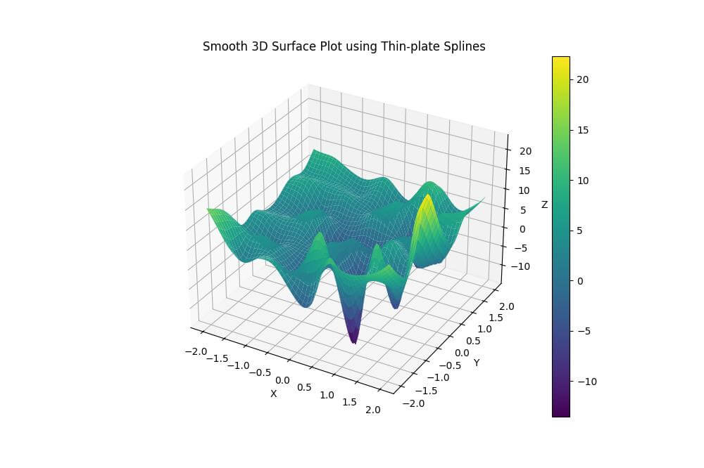
This method minimizes the bending energy of the surface.