3D Blob Shapes in Python (Creation & Manipulation)

In this tutorial, you’ll learn how to create and manipulate 3D blob shapes using Python.

Blob shapes are organic, amorphous forms that can be used in various applications, from computer graphics to scientific visualizations.

You’ll explore different methods to generate, manipulate, and represent these shapes in 3D space.

 

 

Generate Basic 3D Blob Shapes

Using Parametric Equations

To create a basic 3D blob shape using parametric equations, you can use the numpy and matplotlib libraries.

Here’s how you can generate a simple blob:

import numpy as np
import matplotlib.pyplot as plt
from mpl_toolkits.mplot3d import Axes3D
def blob(u, v):
    x = np.cos(u) * (4 + np.sin(2*v))
    y = np.sin(u) * (4 + np.sin(2*v))
    z = 2 * np.cos(v)
    return x, y, z
u = np.linspace(0, 2*np.pi, 100)
v = np.linspace(0, np.pi, 100)
u, v = np.meshgrid(u, v)
x, y, z = blob(u, v)
fig = plt.figure(figsize=(10, 8))
ax = fig.add_subplot(111, projection='3d')
ax.plot_surface(x, y, z, cmap='viridis')
plt.show()

Output:

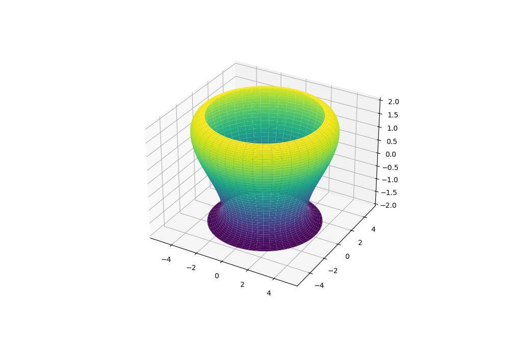
The blob function defines the parametric equations for the shape using trigonometric functions to create an organic form.

The resulting plot shows a rounded, asymmetric shape with undulations on its surface.

Perturbing Primitive Shapes

You can create more complex blob shapes by perturbing primitive shapes like spheres. Here’s an example of how to create a perturbed sphere:

import numpy as np
import matplotlib.pyplot as plt
from mpl_toolkits.mplot3d import Axes3D
def perturbed_sphere(u, v, perturbation=0.3):
    r = 1 + perturbation * np.random.randn(u.shape[0], u.shape[1])
    x = r * np.sin(u) * np.cos(v)
    y = r * np.sin(u) * np.sin(v)
    z = r * np.cos(u)
    return x, y, z
u = np.linspace(0, np.pi, 50)
v = np.linspace(0, 2*np.pi, 50)
u, v = np.meshgrid(u, v)
x, y, z = perturbed_sphere(u, v)
fig = plt.figure(figsize=(10, 8))
ax = fig.add_subplot(111, projection='3d')
ax.plot_surface(x, y, z, cmap='coolwarm')
plt.show()

Output:

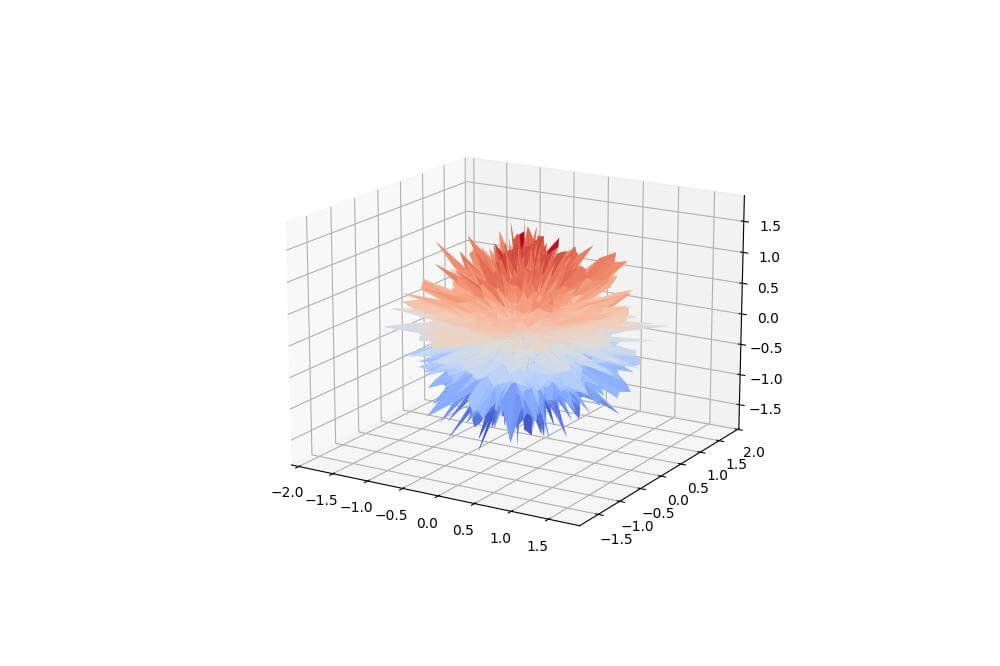
This code creates a perturbed sphere by adding random noise to the radius of a regular sphere.

The resulting plot shows a blob-like shape with irregular bumps and depressions on its surface.

 

Noise-Based Blob Creation (Perlin Noise, Simplex Noise)

You can use noise functions like Perlin noise to create more complex and natural-looking blob shapes. Here’s an example using the noise library:

import numpy as np
import matplotlib.pyplot as plt
from mpl_toolkits.mplot3d import Axes3D
from noise import snoise3
def noise_blob(u, v, scale=1, octaves=4):
    x = np.sin(u) * np.cos(v)
    y = np.sin(u) * np.sin(v)
    z = np.cos(u)
    noise = np.array([snoise3(scale*x, scale*y, scale*z, octaves=octaves) 
                      for x, y, z in zip(x.flatten(), y.flatten(), z.flatten())])
    noise = noise.reshape(x.shape)
    return (1 + 0.5 * noise) * x, (1 + 0.5 * noise) * y, (1 + 0.5 * noise) * z
u = np.linspace(0, np.pi, 100)
v = np.linspace(0, 2*np.pi, 100)
u, v = np.meshgrid(u, v)
x, y, z = noise_blob(u, v)
fig = plt.figure(figsize=(10, 8))
ax = fig.add_subplot(111, projection='3d')
ax.plot_surface(x, y, z, cmap='terrain')
plt.show()

Output:

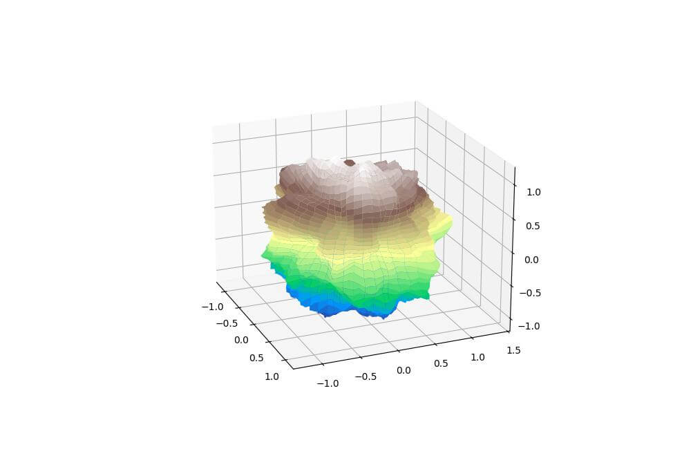
The resulting plot shows a blob with complex surface features.

 

Procedural Blob Generation Using Mathematical Functions

You can create unique blob shapes by combining various mathematical functions.

Here’s an example of a procedurally generated blob:

import numpy as np
import matplotlib.pyplot as plt
from mpl_toolkits.mplot3d import Axes3D
def procedural_blob(u, v):
    r = 1 + 0.3 * np.sin(3*u) * np.cos(4*v) + 0.1 * np.cos(5*u) * np.sin(2*v)
    x = r * np.sin(u) * np.cos(v)
    y = r * np.sin(u) * np.sin(v)
    z = r * np.cos(u)
    return x, y, z
u = np.linspace(0, np.pi, 100)
v = np.linspace(0, 2*np.pi, 100)
u, v = np.meshgrid(u, v)
x, y, z = procedural_blob(u, v)
fig = plt.figure(figsize=(10, 8))
ax = fig.add_subplot(111, projection='3d')
ax.plot_surface(x, y, z, cmap='plasma')
plt.show()

Output:

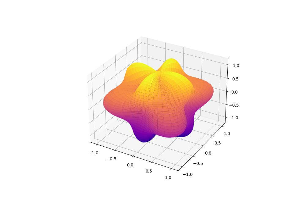
The resulting plot shows a blob with regular patterns of bumps and indentations.

 

Mesh Representation of Blobs

Vertex and Face Data Structures

To represent blob shapes as 3D meshes, you need to define vertex and face data structures. Here’s an example of how to create a simple blob mesh:

import numpy as np
import matplotlib.pyplot as plt
from mpl_toolkits.mplot3d import Axes3D
def create_blob_mesh(resolution=20):
    phi = np.linspace(0, np.pi, resolution)
    theta = np.linspace(0, 2*np.pi, resolution)
    phi, theta = np.meshgrid(phi, theta)

    r = 1 + 0.2 * np.sin(4*phi) * np.cos(4*theta)
    x = r * np.sin(phi) * np.cos(theta)
    y = r * np.sin(phi) * np.sin(theta)
    z = r * np.cos(phi)
    vertices = np.column_stack((x.flatten(), y.flatten(), z.flatten()))
    faces = []
    for i in range(resolution-1):
        for j in range(resolution-1):
            v0 = i * resolution + j
            v1 = v0 + 1
            v2 = (i+1) * resolution + j
            v3 = v2 + 1
            faces.append([v0, v1, v2])
            faces.append([v1, v3, v2])
    return vertices, np.array(faces)
vertices, faces = create_blob_mesh()
fig = plt.figure(figsize=(10, 8))
ax = fig.add_subplot(111, projection='3d')
ax.plot_trisurf(vertices[:, 0], vertices[:, 1], vertices[:, 2], triangles=faces, cmap='viridis')
plt.show()

Output:

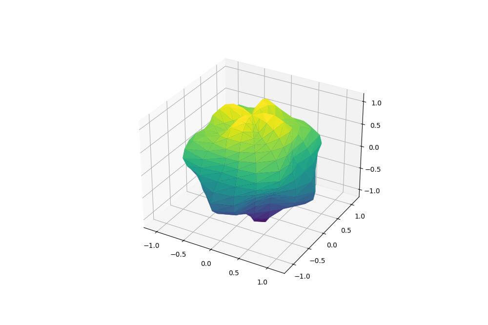
The create_blob_mesh function generates a set of vertices using spherical coordinates with a perturbation function, and then creates triangular faces to connect these vertices.

The resulting plot shows a 3D mesh representation of a blob shape.

Triangulation Methods for Blob Surfaces

For more complex blob shapes, you might need to use advanced triangulation methods.

Here’s an example using Delaunay triangulation:

import numpy as np
import matplotlib.pyplot as plt
from mpl_toolkits.mplot3d import Axes3D
from scipy.spatial import Delaunay
def generate_blob_points(n_points=1000):
    phi = np.random.uniform(0, np.pi, n_points)
    theta = np.random.uniform(0, 2*np.pi, n_points)
    r = 1 + 0.3 * np.random.randn(n_points)

    x = r * np.sin(phi) * np.cos(theta)
    y = r * np.sin(phi) * np.sin(theta)
    z = r * np.cos(phi)
    return np.column_stack((x, y, z))
points = generate_blob_points()
hull = Delaunay(points)
fig = plt.figure(figsize=(10, 8))
ax = fig.add_subplot(111, projection='3d')
ax.plot_trisurf(points[:, 0], points[:, 1], points[:, 2], triangles=hull.simplices, cmap='coolwarm')
plt.show()

Output:

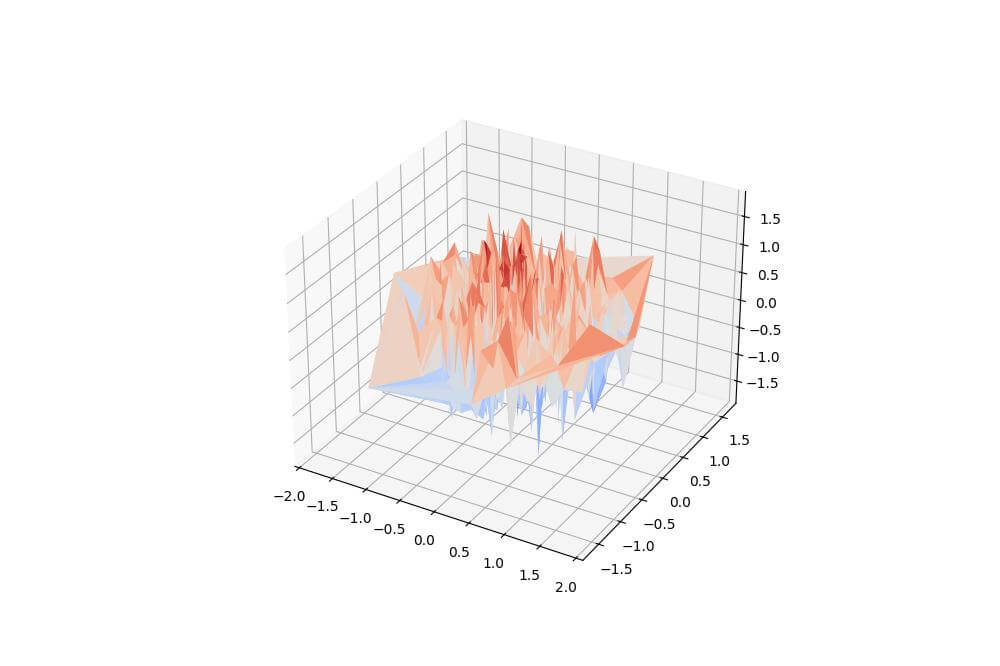
This code generates random points on a perturbed sphere and then uses Delaunay triangulation to create a mesh.

The resulting plot shows a blob-like shape with a more irregular surface compared to the previous example.

 

Scaling, Rotation, and Translation Operations

You can manipulate blob shapes using basic transformations like scaling, rotation, and translation. Here’s an example:

import numpy as np
import matplotlib.pyplot as plt
from mpl_toolkits.mplot3d import Axes3D
def create_blob(u, v):
    x = np.cos(u) * (3 + np.cos(v))
    y = np.sin(u) * (3 + np.cos(v))
    z = np.sin(v)
    return np.column_stack((x.flatten(), y.flatten(), z.flatten()))
def scale(points, sx, sy, sz):
    return points * np.array([sx, sy, sz])
def rotate_z(points, angle):
    c, s = np.cos(angle), np.sin(angle)
    rotation_matrix = np.array([[c, -s, 0], [s, c, 0], [0, 0, 1]])
    return np.dot(points, rotation_matrix.T)
def translate(points, tx, ty, tz):
    return points + np.array([tx, ty, tz])
u = np.linspace(0, 2*np.pi, 50)
v = np.linspace(-np.pi/2, np.pi/2, 50)
u, v = np.meshgrid(u, v)
blob_points = create_blob(u, v)
transformed_points = translate(rotate_z(scale(blob_points, 1.5, 0.8, 1.2), np.pi/4), 1, -1, 0.5)
fig = plt.figure(figsize=(12, 5))
ax1 = fig.add_subplot(121, projection='3d')
ax1.scatter(blob_points[:, 0], blob_points[:, 1], blob_points[:, 2], c=blob_points[:, 2], cmap='viridis', s=10)
ax1.set_title('Original Blob')
ax2 = fig.add_subplot(122, projection='3d')
ax2.scatter(transformed_points[:, 0], transformed_points[:, 1], transformed_points[:, 2], c=transformed_points[:, 2], cmap='viridis', s=10)
ax2.set_title('Transformed Blob')
plt.tight_layout()
plt.show()

Output:

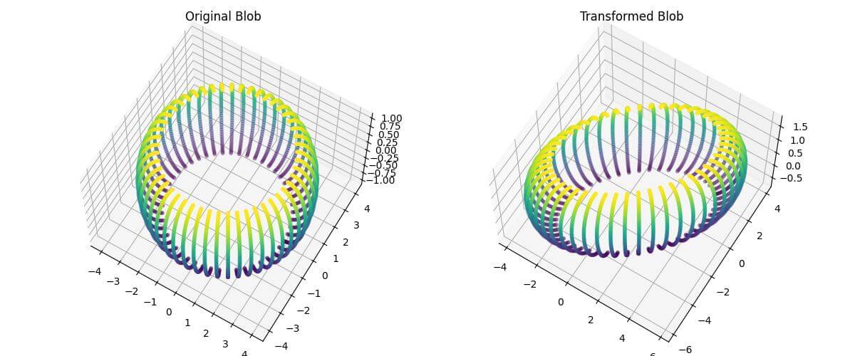
The transformed blob is scaled non-uniformly, rotated around the z-axis, and translated in 3D space.

 

Apply Non-Uniform Deformations

You can create more complex deformations by applying non-uniform transformations to your blob shapes.

Here’s an example of a twist deformation:

import numpy as np
import matplotlib.pyplot as plt
from mpl_toolkits.mplot3d import Axes3D
def create_blob(u, v):
    x = np.cos(u) * (3 + np.cos(v))
    y = np.sin(u) * (3 + np.cos(v))
    z = np.sin(v)
    return np.column_stack((x.flatten(), y.flatten(), z.flatten()))
def twist_deformation(points, twist_factor):
    x, y, z = points[:, 0], points[:, 1], points[:, 2]
    theta = twist_factor * z
    x_new = x * np.cos(theta) - y * np.sin(theta)
    y_new = x * np.sin(theta) + y * np.cos(theta)
    return np.column_stack((x_new, y_new, z))
u = np.linspace(0, 2*np.pi, 50)
v = np.linspace(-np.pi/2, np.pi/2, 50)
u, v = np.meshgrid(u, v)
blob_points = create_blob(u, v)
twisted_points = twist_deformation(blob_points, 0.5)
fig = plt.figure(figsize=(12, 5))
ax1 = fig.add_subplot(121, projection='3d')
ax1.scatter(blob_points[:, 0], blob_points[:, 1], blob_points[:, 2], c=blob_points[:, 2], cmap='viridis', s=10)
ax1.set_title('Original Blob')
ax2 = fig.add_subplot(122, projection='3d')
ax2.scatter(twisted_points[:, 0], twisted_points[:, 1], twisted_points[:, 2], c=twisted_points[:, 2], cmap='viridis', s=10)
ax2.set_title('Twisted Blob')
plt.tight_layout()
plt.show()

Output:

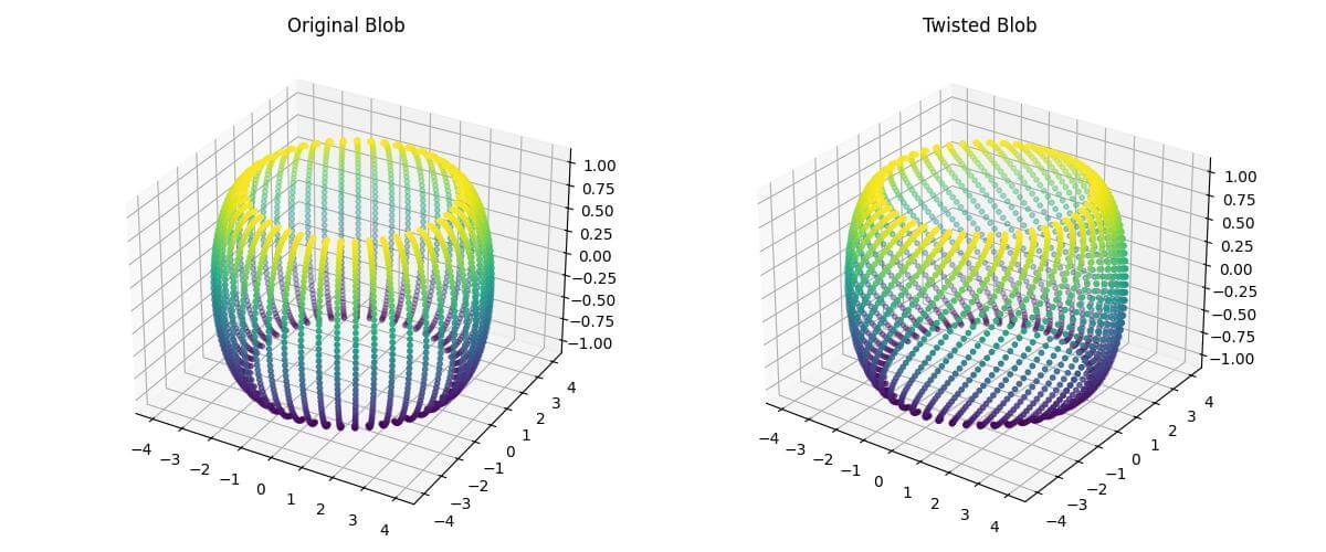
The twist_deformation function rotates each point around the z-axis by an amount proportional to its z-coordinate.