Create 3D Surface Plots with Bicubic Interpolation in Python

In this tutorial, you’ll learn how to create 3D surface plots using bicubic interpolation in Python.

Bicubic interpolation is a powerful method for smoothing the resolution of 3D data.

You’ll use libraries like NumPy, SciPy, and Matplotlib to generate sample data, apply bicubic interpolation, and visualize the results.

 

 

Generate Sample Data

To start, you’ll need to create a grid of X and Y coordinates. Use NumPy to generate this grid:

import numpy as np
x = np.linspace(-5, 5, 10)
y = np.linspace(-5, 5, 10)
X, Y = np.meshgrid(x, y)

This code creates a 10×10 grid of X and Y coordinates ranging from -5 to 5.

Next, define a function to generate Z values based on X and Y coordinates:

def z_func(x, y):
    return np.sin(np.sqrt(x**2 + y**2))
Z = z_func(X, Y)

This function creates a sinusoidal surface based on the distance from the origin.

 

Create the 3D Surface Plot

You can use the RegularGridInterpolator for interpolation on a regular grid:

import numpy as np
from scipy import interpolate
import matplotlib.pyplot as plt
from mpl_toolkits.mplot3d import Axes3D
x = np.linspace(-5, 5, 10)
y = np.linspace(-5, 5, 10)
X, Y = np.meshgrid(x, y)
def z_func(x, y):
    return np.sin(np.sqrt(x**2 + y**2))
Z = z_func(X, Y)
f = interpolate.RegularGridInterpolator((x, y), Z, method='cubic')
x_new = np.linspace(-5, 5, 100)
y_new = np.linspace(-5, 5, 100)
X_new, Y_new = np.meshgrid(x_new, y_new)
Z_new = f((X_new, Y_new))
fig = plt.figure(figsize=(12, 5))
ax1 = fig.add_subplot(121, projection='3d')
ax1.plot_surface(X, Y, Z, cmap='viridis')
ax1.set_title('Original Data')
ax2 = fig.add_subplot(122, projection='3d')
ax2.plot_surface(X_new, Y_new, Z_new, cmap='viridis')
ax2.set_title('Interpolated Data')
plt.tight_layout()
plt.show()

Output:

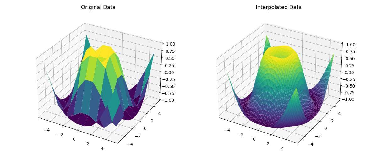
This code creates two subplots: one showing the original data and another showing the interpolated data.

The RegularGridInterpolator is initialized with the original grid and data, and then used to interpolate the new grid points.

 

Handle Edge Cases and Challenges

Deal with Discontinuities in Data

When dealing with discontinuities, you may need to adjust your interpolation method:

def z_func_discontinuous(x, y):
    return np.where(x*y > 0, np.sin(np.sqrt(x**2 + y**2)), 0)
Z_discontinuous = z_func_discontinuous(X, Y)
f_discontinuous = RegularGridInterpolator((x, y), Z_discontinuous, method='cubic')
x_new = np.linspace(-5, 5, 100)
y_new = np.linspace(-5, 5, 100)
X_new, Y_new = np.meshgrid(x_new, y_new)
pts = np.array([X_new.flatten(), Y_new.flatten()]).T
Z_new_discontinuous = f_discontinuous(pts).reshape(X_new.shape)

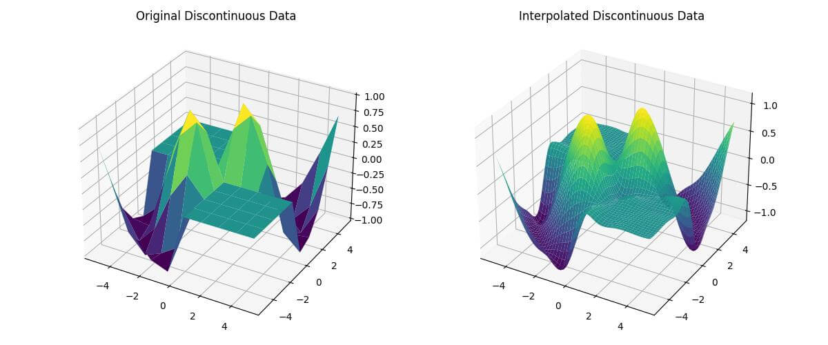
This code creates a discontinuous surface and applies bicubic interpolation.

Let’s visualize both plots:

import numpy as np
import matplotlib.pyplot as plt
from mpl_toolkits.mplot3d import Axes3D
from scipy.interpolate import RegularGridInterpolator

# Generate data with discontinuities
x = np.linspace(-5, 5, 10)
y = np.linspace(-5, 5, 10)
X, Y = np.meshgrid(x, y)
def z_func_discontinuous(x, y):
    return np.where(x*y > 0, np.sin(np.sqrt(x**2 + y**2)), 0)
Z_discontinuous = z_func_discontinuous(X, Y)
f_discontinuous = RegularGridInterpolator((x, y), Z_discontinuous, method='cubic')
x_new = np.linspace(-5, 5, 100)
y_new = np.linspace(-5, 5, 100)
X_new, Y_new = np.meshgrid(x_new, y_new)
pts = np.array([X_new.flatten(), Y_new.flatten()]).T
Z_new_discontinuous = f_discontinuous(pts).reshape(X_new.shape)

fig = plt.figure(figsize=(12, 5))
ax1 = fig.add_subplot(121, projection='3d')
ax1.plot_surface(X, Y, Z_discontinuous, cmap='viridis')
ax1.set_title('Original Discontinuous Data')
ax2 = fig.add_subplot(122, projection='3d')
ax2.plot_surface(X_new, Y_new, Z_new_discontinuous, cmap='viridis')
ax2.set_title('Interpolated Discontinuous Data')
plt.tight_layout()
plt.show()

Output:

Smoothing Noisy Data

When dealing with noisy data, you might want to apply smoothing before interpolation:

from scipy.ndimage import gaussian_filter
Z_noisy = Z_discontinuous + np.random.normal(0, 0.1, Z_discontinuous.shape)

# Apply Gaussian smoothing
Z_smoothed = gaussian_filter(Z_noisy, sigma=1)
interp_func_smoothed = RegularGridInterpolator((x, y), Z_smoothed)
Z_new_smoothed = interp_func_smoothed(pts).reshape(X_new.shape)

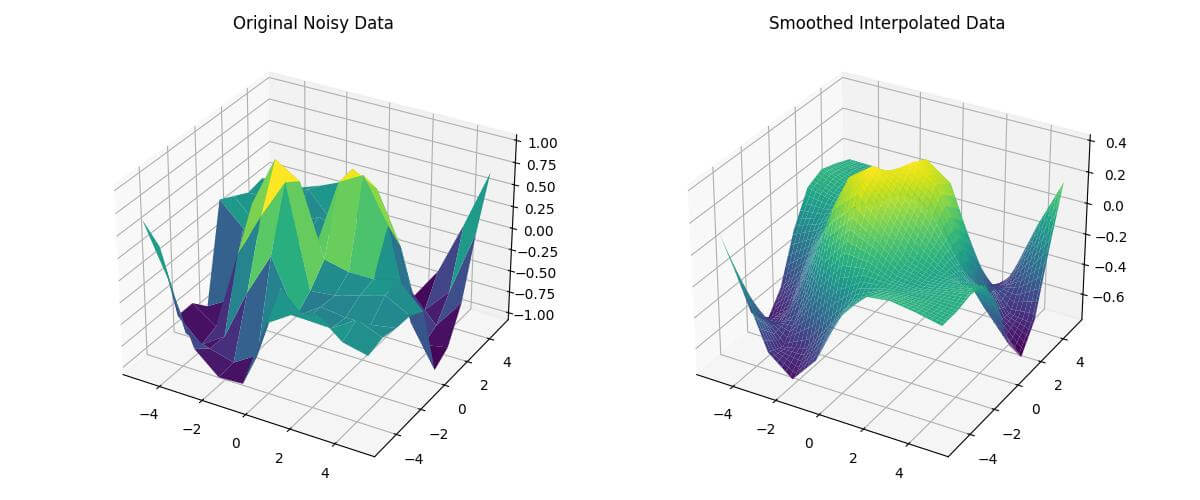
This code adds noise to the original data, applies Gaussian smoothing, and then performs interpolation on the smoothed data.

The smoothed data will be like this:

import matplotlib.pyplot as plt
from mpl_toolkits.mplot3d import Axes3D
from scipy import interpolate
import numpy as np
from scipy.interpolate import RegularGridInterpolator
x = np.linspace(-5, 5, 10)
y = np.linspace(-5, 5, 10)
X, Y = np.meshgrid(x, y)
def z_func_discontinuous(x, y):
    return np.where(x*y > 0, np.sin(np.sqrt(x**2 + y**2)), 0)
Z_discontinuous = z_func_discontinuous(X, Y)
interp_func = RegularGridInterpolator((x, y), Z_discontinuous)
x_new = np.linspace(-5, 5, 100)
y_new = np.linspace(-5, 5, 100)
X_new, Y_new = np.meshgrid(x_new, y_new)
pts = np.array([X_new.flatten(), Y_new.flatten()]).T
Z_noisy = Z_discontinuous + np.random.normal(0, 0.1, Z_discontinuous.shape)

# Apply Gaussian smoothing
Z_smoothed = gaussian_filter(Z_noisy, sigma=1)

# Interpolate smoothed data
interp_func_smoothed = RegularGridInterpolator((x, y), Z_smoothed)
Z_new_smoothed = interp_func_smoothed(pts).reshape(X_new.shape)
fig = plt.figure(figsize=(12, 5))
ax1 = fig.add_subplot(121, projection='3d')
ax1.plot_surface(X, Y, Z_noisy, cmap='viridis')
ax1.set_title('Original Noisy Data')
ax2 = fig.add_subplot(122, projection='3d')
ax2.plot_surface(X_new, Y_new, Z_new_smoothed, cmap='viridis')
ax2.set_title('Smoothed Interpolated Data')
plt.tight_layout()
plt.show()

Output: