How to Plot 3D Vector in Python using Matplotlib

In this tutorial, you’ll learn how to plot 3D vectors in Python using the Matplotlib library.

You’ll learn how to customize vector appearance and perform vector operations.

 

 

Define Vector Components (x, y, z)

To begin, you need to define the components of your 3D vector. Let’s create a sample vector:

x, y, z = 2, 3, 4

To work with vector data, you’ll use NumPy arrays:

import numpy as np
vector = np.array([x, y, z])
print("Vector as NumPy array:", vector)

Output:

Vector as NumPy array: [2 3 4]

The NumPy array representation allows for easier manipulation and plotting of the vector data.

 

Plot using quiver3D

To create a 3D vector plot using quiver3D, you can use the following code:

import matplotlib.pyplot as plt
from mpl_toolkits.mplot3d import Axes3D
fig = plt.figure(figsize=(8, 6))
ax = fig.add_subplot(111, projection='3d')
ax.quiver(0, 0, 0, x, y, z, color='r', arrow_length_ratio=0.1)
ax.set_xlim([0, max(x, y, z)])
ax.set_ylim([0, max(x, y, z)])
ax.set_zlim([0, max(x, y, z)])
ax.set_xlabel('X')
ax.set_ylabel('Y')
ax.set_zlabel('Z')
plt.title('3D Vector Plot using quiver3D')
plt.show()

Output:

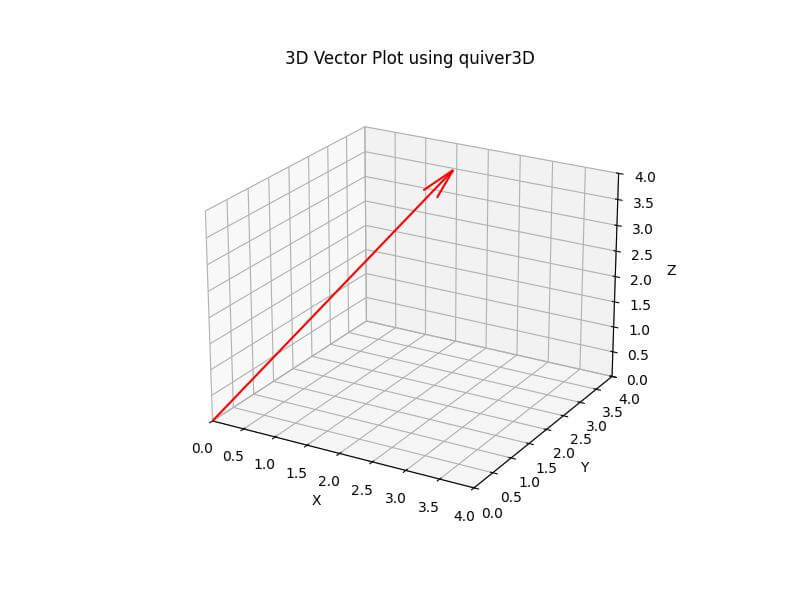
This code creates a 3D plot of the vector using the quiver3D function, which draws an arrow from the origin to the vector’s endpoint.

 

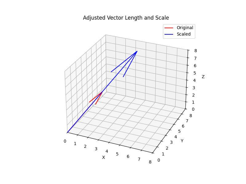
Adjust Vector Length and Scale

To adjust the vector length and scale, you can modify the vector components:

scale_factor = 2
scaled_vector = vector * scale_factor
fig = plt.figure(figsize=(8, 6))
ax = fig.add_subplot(111, projection='3d')
ax.quiver(0, 0, 0, *vector, color='r', label='Original')
ax.quiver(0, 0, 0, *scaled_vector, color='b', label='Scaled')
ax.set_xlim([0, max(scaled_vector)])
ax.set_ylim([0, max(scaled_vector)])
ax.set_zlim([0, max(scaled_vector)])
ax.set_xlabel('X')
ax.set_ylabel('Y')
ax.set_zlabel('Z')
ax.legend()
plt.title('Adjusted Vector Length and Scale')
plt.show()

Output:

 

Set Arrow Properties (width, color, style)

You can customize the arrow properties to enhance the visual representation:

fig = plt.figure(figsize=(8, 6))
ax = fig.add_subplot(111, projection='3d')
ax.quiver(0, 0, 0, x, y, z, color='g', arrow_length_ratio=0.15, linewidth=2, linestyle='--')
ax.set_xlim([0, max(x, y, z)])
ax.set_ylim([0, max(x, y, z)])
ax.set_zlim([0, max(x, y, z)])
ax.set_xlabel('X')
ax.set_ylabel('Y')
ax.set_zlabel('Z')
plt.title('Customized Arrow Properties')
plt.show()

Output:

 

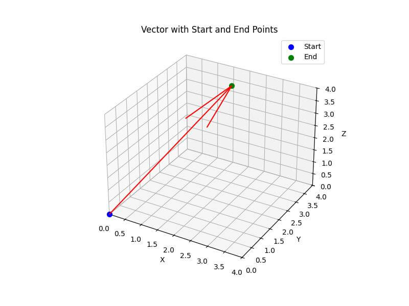
Add Points for Vector Start and End

To highlight the vector’s start and end points, you can add markers:

fig = plt.figure(figsize=(8, 6))
ax = fig.add_subplot(111, projection='3d')
ax.quiver(0, 0, 0, x, y, z, color='r')
ax.scatter(0, 0, 0, color='b', s=50, label='Start')
ax.scatter(x, y, z, color='g', s=50, label='End')
ax.set_xlim([0, max(x, y, z)])
ax.set_ylim([0, max(x, y, z)])
ax.set_zlim([0, max(x, y, z)])
ax.set_xlabel('X')
ax.set_ylabel('Y')
ax.set_zlabel('Z')
ax.legend()
plt.title('Vector with Start and End Points')
plt.show()

Output:

 

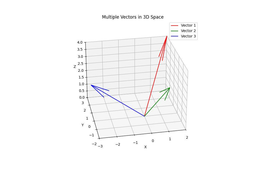
Plot Multiple Vectors

To plot multiple vectors in the same space, you can use the following code:

vectors = np.array([[2, 3, 4], [1, -2, 3], [-3, 1, 2]])
fig = plt.figure(figsize=(10, 8))
ax = fig.add_subplot(111, projection='3d')
colors = ['r', 'g', 'b']
for i, v in enumerate(vectors):
    ax.quiver(0, 0, 0, *v, color=colors[i], label=f'Vector {i+1}')
ax.set_xlim([min(vectors[:, 0].min(), 0), max(vectors[:, 0].max(), 0)])
ax.set_ylim([min(vectors[:, 1].min(), 0), max(vectors[:, 1].max(), 0)])
ax.set_zlim([min(vectors[:, 2].min(), 0), max(vectors[:, 2].max(), 0)])
ax.set_xlabel('X')
ax.set_ylabel('Y')
ax.set_zlabel('Z')
ax.legend()
plt.title('Multiple Vectors in 3D Space')
plt.show()

Output:

 

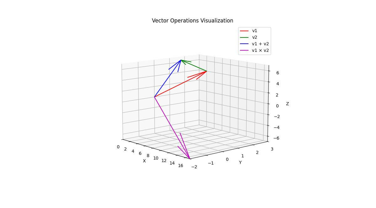
Vector Operations Visualization

To visualize vector operations, you can use the following code:

v1 = np.array([2, 3, 4])
v2 = np.array([1, -2, 3])
fig = plt.figure(figsize=(12, 10))
ax = fig.add_subplot(111, projection='3d')

# Vector addition
v_sum = v1 + v2
ax.quiver(0, 0, 0, *v1, color='r', label='v1')
ax.quiver(*v1, *v2, color='g', label='v2')
ax.quiver(0, 0, 0, *v_sum, color='b', label='v1 + v2')

# Cross product
v_cross = np.cross(v1, v2)
ax.quiver(0, 0, 0, *v_cross, color='m', label='v1 × v2')
ax.set_xlim([min(0, v1[0], v2[0], v_sum[0], v_cross[0]), max(0, v1[0], v2[0], v_sum[0], v_cross[0])])
ax.set_ylim([min(0, v1[1], v2[1], v_sum[1], v_cross[1]), max(0, v1[1], v2[1], v_sum[1], v_cross[1])])
ax.set_zlim([min(0, v1[2], v2[2], v_sum[2], v_cross[2]), max(0, v1[2], v2[2], v_sum[2], v_cross[2])])
ax.set_xlabel('X')
ax.set_ylabel('Y')
ax.set_zlabel('Z')
ax.legend()
plt.title('Vector Operations Visualization')
plt.show()

# Dot product
dot_product = np.dot(v1, v2)
print(f"Dot product of v1 and v2: {dot_product}")

Output:

Dot product of v1 and v2: 8

This code visualizes vector addition and the cross product of two vectors in 3D space.

It also calculates and prints the dot product of the vectors.