Create 3D Surface Plot Using 2D Array in Python

In this tutorial, you’ll learn how to create 3D surface plots using 2D arrays in Python.

You’ll use the Matplotlib library to bring your data to life in three dimensions.

 

 

Using plot_surface()

To create a basic 3D surface plot, you can use the plot_surface() function from the Matplotlib mplot3d toolkit.

import numpy as np
import matplotlib.pyplot as plt
from mpl_toolkits.mplot3d import Axes3D
x = np.linspace(-5, 5, 50)
y = np.linspace(-5, 5, 50)
X, Y = np.meshgrid(x, y)
Z = np.sin(np.sqrt(X**2 + Y**2))
fig = plt.figure(figsize=(10, 8))
ax = fig.add_subplot(111, projection='3d')
surf = ax.plot_surface(X, Y, Z)
ax.set_xlabel('X axis')
ax.set_ylabel('Y axis')
ax.set_zlabel('Z axis')
ax.set_title('3D Surface Plot: sin(sqrt(x^2 + y^2))')
plt.show()

Output:

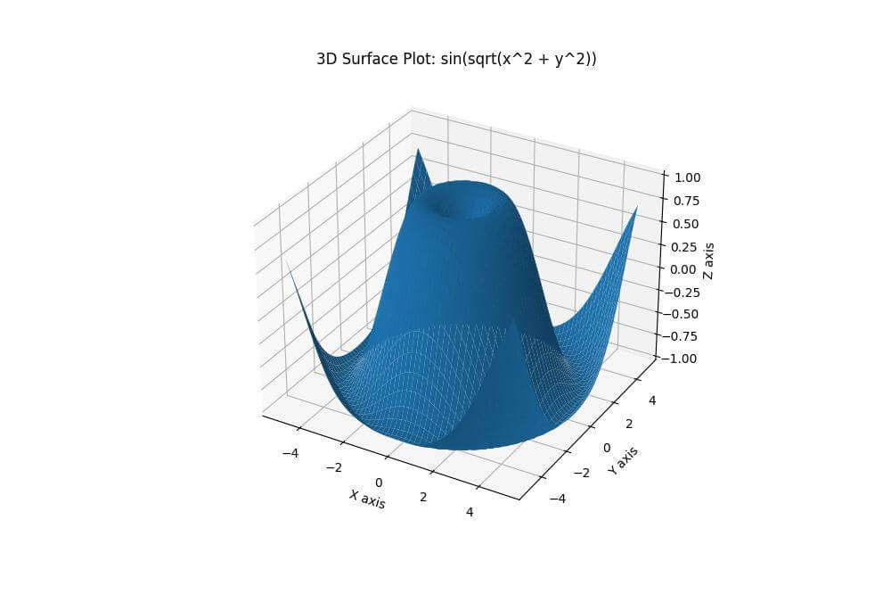
This code creates a 3D surface plot of the function sin(sqrt(x^2 + y^2)).

Here, Z is computed as the sine of the square root of the sum of squares of X and Y.

 

Using plot_wireframe()

For a different perspective on your 3D data, you can create a wireframe plot using the plot_wireframe() function.

amr = np.linspace(-3, 3, 30)
fatma = np.linspace(-3, 3, 30)
AMR, FATMA = np.meshgrid(amr, fatma)
HASSAN = np.sin(AMR) * np.cos(FATMA)
fig = plt.figure(figsize=(10, 8))
ax = fig.add_subplot(111, projection='3d')
wire = ax.plot_wireframe(AMR, FATMA, HASSAN, rstride=2, cstride=2)
ax.set_xlabel('Amr')
ax.set_ylabel('Fatma')
ax.set_zlabel('Hassan')
ax.set_title('3D Wireframe Plot: sin(x) * cos(y)')
plt.show()

Output:

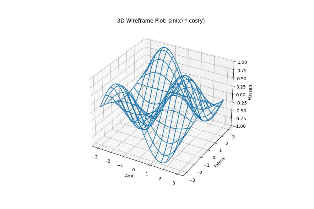
This code creates a wireframe plot of the function sin(x) * cos(y).

The resulting plot shows a 3D grid structure that outlines the shape of the function.

 

Using contour3D()

To create a 3D contour plot, you can use the contour3D() function, which draws contour lines on a 3D surface.

nour = np.linspace(-3, 3, 50)
ahmed = np.linspace(-3, 3, 50)
NOUR, AHMED = np.meshgrid(nour, ahmed)
MOHAMED = (1 - NOUR**2 + AHMED**3) * np.exp(-(NOUR**2 + AHMED**2) / 2)
fig = plt.figure(figsize=(10, 8))
ax = fig.add_subplot(111, projection='3d')
cont = ax.contour3D(NOUR, AHMED, MOHAMED, 50, cmap='coolwarm')
ax.set_xlabel('Nour')
ax.set_ylabel('Ahmed')
ax.set_zlabel('Mohamed')
ax.set_title('3D Contour Plot')
plt.show()

Output:

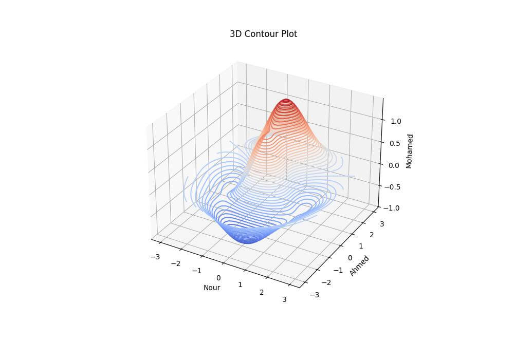
This code creates a 3D contour plot of a more complex function.

The resulting plot shows contour lines drawn on a 3D surface, with colors representing different levels of the Z values.

 

Using contourf3D()

For a filled 3D contour plot, you can use the contourf3D() function, which creates a plot with colored regions between contour levels.

samir = np.linspace(-2, 2, 40)
laila = np.linspace(-2, 2, 40)
SAMIR, LAILA = np.meshgrid(samir, laila)
YARA = SAMIR * np.exp(-SAMIR**2 - LAILA**2)
fig = plt.figure(figsize=(10, 8))
ax = fig.add_subplot(111, projection='3d')
cont_filled = ax.contourf3D(SAMIR, LAILA, YARA, 50, cmap='viridis')
fig.colorbar(cont_filled, shrink=0.6, aspect=8)
ax.set_xlabel('Samir')
ax.set_ylabel('Laila')
ax.set_zlabel('Yara')
ax.set_title('Filled 3D Contour Plot')
plt.show()

Output:

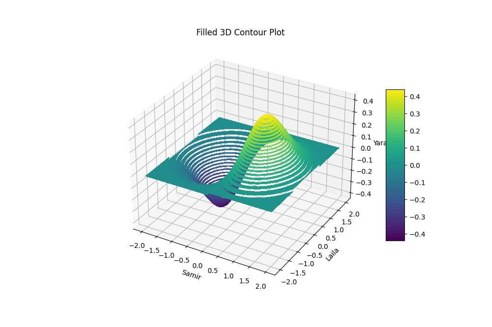
This code creates a filled 3D contour plot of the function x * exp(-x^2 – y^2).

The resulting plot shows colored regions representing different ranges of Z values.