How to Plot 3D Polygon in Python using Matplotlib

In this tutorial, you’ll learn how to plot 3D polygons in Python using the Matplotlib library.

You’ll create complex 3D shapes, handle various polygon types, and implement advanced methods for rendering multiple polygons.

 

 

Create 3D Polygon Vertices

To begin, you’ll need to define the vertices of your 3D polygon. Here’s how you can create a simple 3D polygon:

import numpy as np
import matplotlib.pyplot as plt
from mpl_toolkits.mplot3d import Axes3D
vertices = np.array([
    [0, 0, 0],
    [1, 0, 0],
    [1, 1, 0],
    [0, 1, 0],
    [0.5, 0.5, 1]
])
print(vertices)

Output:

[[0.  0.  0. ]
 [1.  0.  0. ]
 [1.  1.  0. ]
 [0.  1.  0. ]
 [0.5 0.5 1. ]]

This code creates a 3D pyramid with a square base and a point at the top.

NumPy arrays provide an efficient way to store and manipulate large sets of vertices:

t = np.linspace(0, 2*np.pi, 20)
x = np.cos(t)
y = np.sin(t)
z = np.linspace(0, 2, 20)
vertices = np.column_stack((x, y, z))
print(vertices[:5])

Output:

 [0.94581724 0.32469947 0.10526316]
 [0.78914051 0.61421271 0.21052632]
 [0.54694816 0.83716648 0.31578947]
 [0.24548549 0.96940027 0.42105263]]

This code generates a 3D spiral shape using NumPy functions.

The vertices are created using parametric equations and stacked into a single array.

 

Implement Polygon Faces

To create a 3D polygon, you need to define how the vertices connect to form faces:

faces = [
    [0, 1, 4],
    [1, 2, 4],
    [2, 3, 4],
    [3, 0, 4],
    [0, 1, 2, 3]
]
print(faces)

Output:

[[0, 1, 4], [1, 2, 4], [2, 3, 4], [3, 0, 4], [0, 1, 2, 3]]

This code defines the faces of the pyramid. Each row in the faces array represents a polygon face, with the numbers corresponding to the indices of the vertices.

You can handle both convex and concave polygons by carefully defining the face connectivity:

concave_vertices = np.array([
    [0, 0, 0],
    [1, 0, 0],
    [1, 1, 0],
    [0.5, 0.5, 0],
    [0, 1, 0],
    [0.5, 0.5, 1]
])
concave_faces = np.array([
    [0, 1, 3],
    [1, 2, 3],
    [3, 4, 0],
    [0, 1, 5],
    [1, 2, 5],
    [2, 3, 5],
    [3, 4, 5],
    [4, 0, 5]
])

print("Concave vertices:")
print(concave_vertices)
print("\nConcave faces:")
print(concave_faces)

Output:

Concave vertices:
[[0.  0.  0. ]
 [1.  0.  0. ]
 [1.  1.  0. ]
 [0.5 0.5 0. ]
 [0.  1.  0. ]
 [0.5 0.5 1. ]]

Concave faces:
[[0 1 3]
 [1 2 3]
 [3 4 0]
 [0 1 5]
 [1 2 5]
 [2 3 5]
 [3 4 5]
 [4 0 5]]

This code creates a concave 3D shape by carefully defining the vertices and faces.

The concave part is created by adding a vertex in the middle of the base square.

 

Plot the Polygon

To visualize your 3D polygon, you can use Matplotlib plot_trisurf function:

fig = plt.figure()
ax = fig.add_subplot(111, projection='3d')
ax.plot_trisurf(vertices[:, 0], vertices[:, 1], vertices[:, 2], triangles=faces)
ax.set_xlabel('X')
ax.set_ylabel('Y')
ax.set_zlabel('Z')
plt.title('3D Polygon using plot_trisurf')
plt.show()

Output:

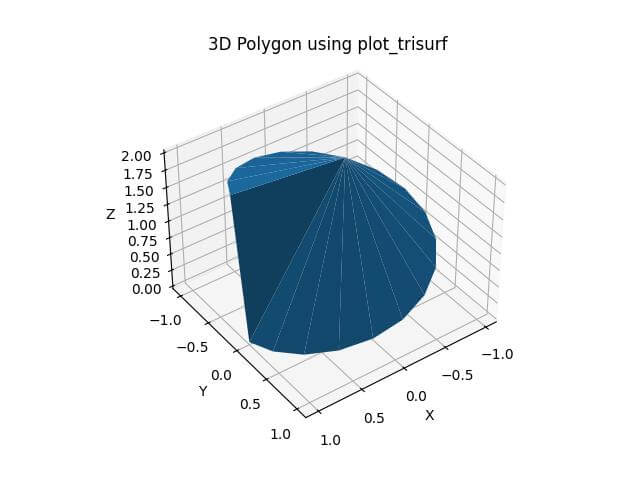
The triangles parameter specifies the face connectivity.

 

Plot Multiple 3D Polygons

To render multiple 3D polygons, you can create separate arrays for each polygon and plot them together:

# Create two 3D polygons
vertices1 = np.array([
    [0, 0, 0],
    [1, 0, 0],
    [1, 1, 0],
    [0, 1, 0],
    [0.5, 0.5, 1]
])
vertices2 = np.array([
    [1.5, 1.5, 0],
    [2.5, 1.5, 0],
    [2.5, 2.5, 0],
    [1.5, 2.5, 0],
    [2, 2, 1]
])
faces = np.array([
    [0, 1, 4],
    [1, 2, 4],
    [2, 3, 4],
    [3, 0, 4],
    [0, 1, 2]
])
fig = plt.figure()
ax = fig.add_subplot(111, projection='3d')
ax.plot_trisurf(vertices1[:, 0], vertices1[:, 1], vertices1[:, 2], triangles=faces, color='r', alpha=0.5)
ax.plot_trisurf(vertices2[:, 0], vertices2[:, 1], vertices2[:, 2], triangles=faces, color='b', alpha=0.5)
ax.set_xlabel('X')
ax.set_ylabel('Y')
ax.set_zlabel('Z')
plt.title('Multiple 3D Polygons')
plt.show()

Output:

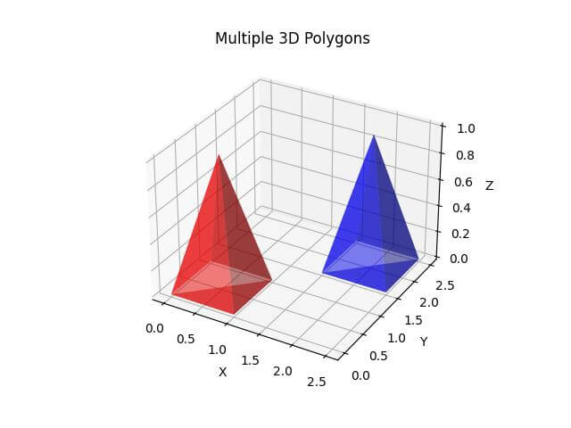
The alpha parameter is used to make the polygons semi-transparent.

 

Plot Quadrilateral

To begin, you’ll create a 3D quadrilateral using Matplotlib Poly3DCollection.

import numpy as np
import matplotlib.pyplot as plt
from mpl_toolkits.mplot3d import Axes3D
from mpl_toolkits.mplot3d.art3d import Poly3DCollection
vertices = np.array([
    [0, 0, 0],
    [1, 0, 0],
    [1, 1, 1],
    [0, 1, 1]
])
fig = plt.figure()
ax = fig.add_subplot(111, projection='3d')

# Create the quadrilateral
quad = [vertices]
poly = Poly3DCollection(quad, alpha=0.8, edgecolor='k')
poly.set_facecolor('cyan')

# Add the quadrilateral to the plot
ax.add_collection3d(poly)
ax.set_xlim(0, 1)
ax.set_ylim(0, 1)
ax.set_zlim(0, 1)
ax.set_xlabel('X')
ax.set_ylabel('Y')
ax.set_zlabel('Z')
plt.title('3D Quadrilateral')
plt.show()

Output:

The quadrilateral is rendered using a cyan color with a slight transparency.

 

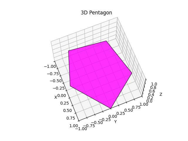
Plot Pentagon

Now, you’ll create a 3D pentagon using trigonometric functions to calculate its vertices.

import numpy as np
import matplotlib.pyplot as plt
from mpl_toolkits.mplot3d import Axes3D
from mpl_toolkits.mplot3d.art3d import Poly3DCollection

# Calculate vertices of a regular pentagon
n_sides = 5
r = 1
vertices = np.array([[r * np.cos(2 * np.pi * i / n_sides),
                      r * np.sin(2 * np.pi * i / n_sides),
                      i * 0.2] for i in range(n_sides)])
fig = plt.figure()
ax = fig.add_subplot(111, projection='3d')
pentagon = [vertices]
poly = Poly3DCollection(pentagon, alpha=0.8, edgecolor='k')
poly.set_facecolor('magenta')
ax.add_collection3d(poly)
ax.set_xlim(-1, 1)
ax.set_ylim(-1, 1)
ax.set_zlim(0, 1)
ax.set_xlabel('X')
ax.set_ylabel('Y')
ax.set_zlabel('Z')
plt.title('3D Pentagon')
plt.show()

Output:

 

Plot Hexagon

Let’s create a 3D hexagon using a similar method to the pentagon but with a different color and orientation.

import numpy as np
import matplotlib.pyplot as plt
from mpl_toolkits.mplot3d import Axes3D
from mpl_toolkits.mplot3d.art3d import Poly3DCollection
n_sides = 6
r = 1
vertices = np.array([[r * np.cos(2 * np.pi * i / n_sides),
                      r * np.sin(2 * np.pi * i / n_sides),
                      np.sin(i * np.pi / 3)] for i in range(n_sides)])
fig = plt.figure()
ax = fig.add_subplot(111, projection='3d')
hexagon = [vertices]
poly = Poly3DCollection(hexagon, alpha=0.8, edgecolor='k')
poly.set_facecolor('gold')
ax.add_collection3d(poly)
ax.set_xlim(-1, 1)
ax.set_ylim(-1, 1)
ax.set_zlim(-1, 1)
ax.set_xlabel('X')
ax.set_ylabel('Y')
ax.set_zlabel('Z')
plt.title('3D Hexagon')
plt.show()

Output:

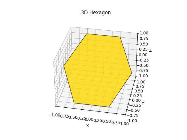
The plot is centered around the origin, with all axes ranging from -1 to 1.

 

Plot Octagon

Now, you’ll create a 3D octagon with a gradient color effect.

import numpy as np
import matplotlib.pyplot as plt
from mpl_toolkits.mplot3d import Axes3D
from mpl_toolkits.mplot3d.art3d import Poly3DCollection
n_sides = 8
r = 1
vertices = np.array([[r * np.cos(2 * np.pi * i / n_sides),
                      r * np.sin(2 * np.pi * i / n_sides),
                      0.5 * np.cos(4 * np.pi * i / n_sides)] for i in range(n_sides)])
fig = plt.figure()
ax = fig.add_subplot(111, projection='3d')
octagon = [vertices]
poly = Poly3DCollection(octagon, alpha=0.8, edgecolor='k')
colors = plt.cm.viridis(np.linspace(0, 1, n_sides))
poly.set_facecolor(colors)
ax.add_collection3d(poly)
ax.set_xlim(-1, 1)
ax.set_ylim(-1, 1)
ax.set_zlim(-0.5, 0.5)
ax.set_xlabel('X')
ax.set_ylabel('Y')
ax.set_zlabel('Z')
plt.title('3D Octagon')
plt.show()

Output:

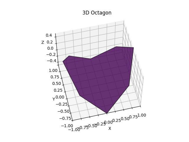
The plot is centered around the origin, with the x and y axes ranging from -1 to 1, and the z-axis from -0.5 to 0.5.