Quicksort algorithm in Python (Step By Step)

In the world of programming, the answers to most of your questions will be found within the data stored in various data structures and with the help of some of the standard algorithms.

Today, we’ll discuss the Quicksort algorithm and how to implement it in Python.

Before you begin on your journey to identifying those answers, you will need a set of data, in many cases sorted data, to perform further computation.

 

 

Sorting algorithms in Python

Sorting involves arranging the data based on certain computational operations, most commonly those greater than (>), or less than (<) operations.

It allows for the arrangement of data in a specific manner, which helps in optimizing the various data-centric operations such as searching.

Sorting can serve multiple purposes, from helping data to be more readable to contributing to faster and optimized programs.

There are several sorting algorithms available that can be implemented in Python. Some of them are:

1. Bubble Sort
   • Time Complexity: Best Case = Ω(N), Worst Case = O(N²), Average Case = Θ(N²)
   • Space Complexity: Worst Case = O(1)
2. Selection Sort
   • Time Complexity: Best Case = Ω(N²), Worst Case = O(N²), Average Case = Θ(N²)
   • Space Complexity: Worst Case = O(1)
3. Heap Sort
   • Time Complexity: Best Case = Ω(NlogN), Worst Case = O(NlogN), Average Case = Θ(NlogN)
   • Space Complexity: Worst Case = O(1)
4. Merge Sort
   • Time Complexity: Best Case = Ω(NlogN), Worst Case = O(NlogN), Average Case = Θ(NlogN)
   • Space Complexity: Worst Case = O(N)
5. Insertion Sort
   • Time Complexity: Best Case = Ω(N), Worst Case = O(N²), Average Case = Θ(N²)
   • Space Complexity: Worst Case = O(1)
6. Quicksort
   • Time Complexity: Best Case = Ω(NlogN), Worst Case = O(N²), Average Case = Θ(NlogN)
   • Space Complexity: Worst Case = O(logN)

Each of these algorithms uses a different approach to perform sorting, resulting in a different time and space complexity.

Each one of them can be used based on the requirements of the program and the availability of resources.
Among those listed, the Quicksort algorithm is considered the fastest because for most inputs, in the average case, Quicksort is found to be the best performing algorithm.

 

Definition

The Quicksort algorithm works on the principle of ‘Divide and Conquer’ to reach a solution.
In each step, we select an element from the data called a ‘pivot’ and determine its correct position in the sorted array.
At the end of the iteration, all the elements to the left of the pivot are less than or equal to the pivot, and all those on the right are greater than the pivot.

The input list is thus partitioned, based on the pivot value, into the left(smaller) list and right(greater) list.
We repeat the process recursively on the left and right sub-arrays until a sorted list is obtained.

In-Place algorithms

Algorithms that do not require extra memory to produce the output, but instead perform operations on the input ‘in-place’ to produce the output are known as ‘in-place algorithms’.
However, a constant space that is extra and generally smaller than linear(O(n)) space can be used for variables.
In the Quicksort algorithm, as the input elements are simply rearranged and manipulated in-place to form the ‘high’ and ‘low’ lists around the pivot and a small constant space is used for certain computations, it is an in-place algorithm.

 

How does Quicksort Works?

Let us break down the Quicksort process into a few steps.

1. Select a pivot.
2. Initialize the left and right pointers, pointing to the left and right ends of the list.
3. Start moving the left and right pointers toward the pivot while their values are smaller and greater than the pivot, respectively.
4. At each step, check and place the elements smaller than the pivot to the left of the pivot, and elements greater than that to the right.
5. When the two pointers meet or cross each other, we have completed one iteration of the list and the pivot is placed in its correct position in the final sorted array.
6. Now, two new lists are obtained on either side of the pivot.
   Repeat steps 1–5 on each of these lists until all elements are placed in their correct positions.

 

QuickSort: The Algorithm

The above process can be expressed as a formal algorithm for Quicksort.
We will perform ‘QUICKSORT’ until elements are present in the list.

A=array

start=lower bound of the array

end = upper bound of the array

pivot= pivot element

 

1. QUICKSORT (array A, start, end)

2. {

3.  if (start >= 0 && start >= 0 && start < end)

4.  {

5.    p = partition(A, start, end)

6.    QUICKSORT(A, start, p)

7.    QUICKSORT(A, p + 1, end)

8.  }

9. }

Observe that the fifth step calls a function called partition.
It is this function that we will use to place the elements on either side of the pivot.
Let’s take a look at it.

1. PARTITION (array A, start, end) 

2. { 

3.  pivot = A[(start+end)//2] 

4.  i = start 

5.  j = end 

6.  while (True) 

7.  {

8.    do i =i + 1 while A[i]<pivot 

9.    do j =j - 1 while A[j]>pivot 

10.   if i>=j then return j 

11.   swap A[i] with A[j] 

12. }

13. } 

In the partition function, we start by assigning an element of the array (here middle element) to the pivot variable.
Variables i and j are used as left and right pointers, they iterate over the array and are used to swap values where needed.
We use the while loop, along with with the return statement, to ensure that the entire array

Let us understand this process with an example.
Take the array A = 3 7 8 5 2 1 9 5 4.
Any element can be chosen as the pivot, but for the purpose of this example, I am taking the middle element.

 

Step 1

start =0, end =8, i=0, j=8, pivot=2
Since a[i]<pivot is false, do nothing, i=0.
a[j] > pivot is true, j-=1. Repeating this until a[j] > pivot, j = 5.
Swap A[i] with A[j] i.e 3 with 1.
So A = 1 7 8 5 2 3 9 5 4, i = 0, j = 5

 

Step 2

i=1, j=4, pivot=2
Since a[i]<pivot is false, do nothing.
Since a[j] > pivot is false, do nothing.
Swap A[i] with A[j] i.e 7 with 2.
So A = 1 2 8 5 7 3 9 5 4, i = 1, j = 4

 

Step 3

i=2, j=3, pivot=2
Since a[i]<pivot is false, do nothing.
Since a[j] > pivot is true, j-=1. Repeating this and stopping at j=1
Since i=2 > j, exit the while loop and return j=1.

At this step, pivot value 2 is in its correct position in the final sorted array.

We now repeat the above steps on two sub-arrays, one with start=0, end=1, and the other with start=2, end=8.

 

Implementation

Let us first define the partition function in Python.

def partition(A, start, end):
    i = start-1 #left pointer
    pivot = A[(start+end)//2] # pivot
    print(f"Pivot = {pivot}")
    j = end+1 #right pointer
    while True:
        i+=1
        while (A[i] < pivot):
            i+=1 #move left pointer to right
        j-=1
        while (A[j]> pivot):
            j-=1 #move right pointer to left
        if i>=j:
            return j #stop, pivot moved to its correct position
        A[i], A[j] = A[j], A[i] 
a = [3,7,8,5,2,4]
print(f"Input array: {a}")
p = partition(a,0,len(a)-1)
print(f"Array after partitioning:{a}")

Output:

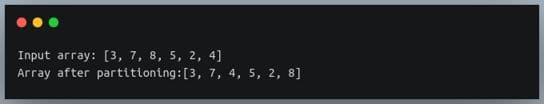
Note how the pivot 8 is moved from its original position 2 to its correct position in the end, such that all elements to its left i.e [0:4] are less than or equal to 8.

This partitioning technique is called ‘Hoare partitioning’, it is the more efficient approach to partitioning.
The other one is called ‘Lomuto partitioning’.

Now let us look at the complete implementation of Quicksort in Python using this partition function.

def quickSort(A, start, end):
    if start < end:
        p = partition(A, start, end) # p is pivot, it is now at its correct position
        # sort elements to left and right of pivot separately
        quickSort(A, start, p)
        quickSort(A, p+1, end)
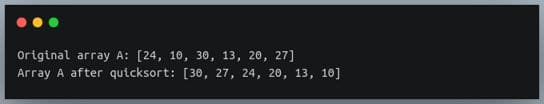
A = [24, 10, 30, 13, 20, 27]
print(f"Original array A: {A}")
quickSort(A, 0, len(A)-1)
print(f"Array A after quicksort: {A}")

Output:

 

Quicksort Time Complexity

For an input of size n, it is divided into parts k and n-k at each step.
So, Time complexity for n elements = Time complexity for k elements + Time complexity for n-k elements + Time complexity for selecting the pivot
i.e T(n)=T(k)+T(n-k)+M(n)

 

Best Case

The best-case complexity occurs when the middle element is selected as the pivot in each recursive loop.
The array is divided into lists of equal size at each iteration and as this process is repeated, the sorting is completed in the minimum number of steps possible.
The number of recursions performed will be log(n) with n operations at each step.
Hence, the time complexity is obtained to be O(n(log(n)).

 

Worst Case

In the worst-case scenario, n number of recursion operations are performed and the time complexity is O(n²).
This can occur under the following conditions:

1. The smallest or largest element is selected as a pivot at each step.
2. The last element is selected as the pivot and the list is already in increasing or decreasing order.

The time complexity can also be found using the master’s theorem.

 

Average Case

The average case is obtained by considering an average of the time complexities of the various permutations of the array. The complexity is O(nlog(n)).

 

Quicksort for descending order

The implementation above leads to the array being sorted in ascending order.
The array can also be sorted in descending order with some changes in the swap condition.
Instead of swapping the left elements when they are greater than the pivot, a swap should be performed when they are smaller than the pivot.
Similarly, instead of swapping the right elements when they are smaller than the pivot, a swap should be performed when they are greater than the pivot.
As a result, a list of elements greater than the pivot will be created to its left and a subarray of elements smaller than the pivot will be created to its right.
Eventually, the array will be arranged in the greatest to smallest order from left to right.

 

Implementation

def partition_desc(A, start, end):
    i = start-1 #left pointer
    pivot = A[(start+end)//2] # pivot
    j = end+1 #right pointer
    while True:
        i+=1
        while (A[i] > pivot):
            i+=1 #move left pointer to right
        j-=1
        while (A[j]< pivot):
            j-=1 #move right pointer to left
        if i>=j:
            return j #stop, pivot moved to its correct position
        A[i], A[j] = A[j], A[i] 
a = [3,7,8,5,2,4]
print(f"Input array: {a}")
p = partition_desc(a,0,len(a)-1)
print(f"Array after partitioning:{a}")

Output:

Now the partition step ensures that the pivot is moved to its correct position in the final descending-order sorted array.
Let us now look at the full Quicksort implementation of the same.

def quickSort_desc(A, start, end):
    if len(A) == 1:
        return A
    if start < end:
        p = partition_desc(A, start, end) # p is pivot, it is now at its correct position
        # sort elements to left and right of pivot separately
        quickSort_desc(A, start, p-1)
        quickSort_desc(A, p+1, end)
A = [24, 10, 30, 13, 20, 27]
print(f"Original array A: {A}")
quickSort_desc(A, 0, len(A)-1)
print(f"Array A after quicksort: {A}")

Output:

 

Quicksort Space Complexity

In the Quicksort algorithm, the partitioning is done in place.
This requires O(1) space.
The elements are then recursively sorted and for each recursive call, a new stack frame of a constant size is used.
The places the space complexity at O(log(n)) in the average case.
This can go up to O(n) for the worst case.

 

Iterative implementation of QuickSort

So far, we have seen the recursive implementation of the Quicksort algorithm. The same can be done in an iterative approach.
In the iterative implementation of Python, the partition function, which performs the comparison and swapping of elements remains the same.
Changes are made to the code in the quicksort function to use a stack implementation instead of recursive calls to the quicksort function.
This works as a temporary stack is created and the first and the last index of the array are placed in it.
Then, the elements are popped from the stack while it is not empty.

Let us look at the code implementation of the same in Python.

def quickSortIterative(A, start, end):
    # Create and initialize the stack, the last filled index represents top of stack
    size = end - start + 1
    stack = [0] * (size)
    top = -1
    # push initial values  to stack
    top = top + 1
    stack[top] = start
    top = top + 1
    stack[top] = end
    # Keep popping from stack while it is not empty
    while top >= 0:
        # Pop start and end
        end = stack[top]
        top = top - 1
        start = stack[top]
        top = top - 1
        # Call the partition step as before
        p = partition( A, start, end )
        # If the left of pivot is not empty,
        # then push left side indices to stack
        if p-1 > start:
            top = top + 1
            stack[top] = start
            top = top + 1
            stack[top] = p - 1
        # If the right of pivot is not empty,
        # then push the right side indices to stack
        if p + 1 < end:
            top = top + 1
            stack[top] = p + 1
            top = top + 1
            stack[top] = end
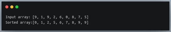
A = [9,1,9,2,6,0,8,7,5]
print(f"Input array: {A}")
n = len(A)
quickSortIterative(A, 0, n-1)
print (f"Sorted array:{A}")

Output:

The elements are popped from the stack while it is not empty.
Within this while loop, the pivot element is moved to its correct position with the help of the partition function.
The stack is used to track the low and high lists with the help of indices of the first and last element.
Two elements popped from the top of the stack represent the start and end indices of a sublist.
Quicksort is implemented iteratively on the lists formed until the stack is empty and the sorted list is obtained.

 

Efficiency of Quicksort

The Quicksort algorithm has better efficiency when the dataset size is small.
As the size of the dataset increases, the efficiency decreases and for larger sets, different sorting algorithms such as merge sort might be more efficient.